A grid that changes every month, planned once a year

The cadence problem #

Most formal planning in the Indian power sector runs on an annual cycle. Resource adequacy filings, capacity plans and tariff petitions are prepared once a year against a set of assumptions fixed at the start of the exercise. That cadence made sense when the quantity being planned changed slowly.

I wanted to know how much the system actually changes inside one of those cycles. The answer is enough to matter.

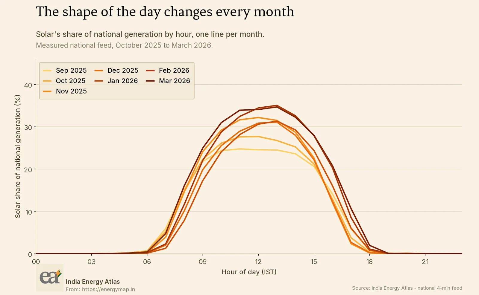
Each line is one month of the measured national feed, plotting solar's share of generation by hour. The lines do not sit on top of each other. Both the height of the midday block and the width of the daylight window move month to month, driven by the seasonal path of the sun, the monsoon, and capacity commissioned during the period.

A plan built on the October shape describes a system that no longer exists by March.

What the dispatchable fleet is asked to do #

The consequence lands on the units that have to fill the gap.

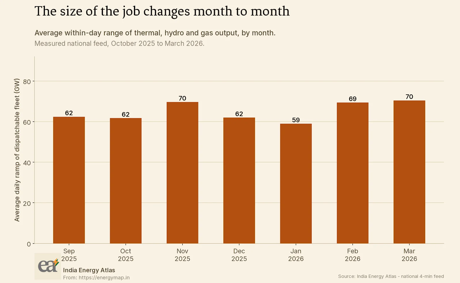
This measures the average within-day range of thermal, hydro and gas output combined, by month. It is the size of the job the dispatchable fleet performs on a typical day in that month. The number is large in absolute terms, and it varies substantially across a six-month window.

A fleet sized and scheduled against the annual average of this quantity will be comfortable in some months and stretched in others. Maintenance planning, coal stocking and unit commitment all depend on which months those are, and an annual model that reports a single figure cannot tell a planner where in the year the pressure falls.

An annual answer to a monthly question answers a different question, and answers it confidently.

Why more analysts is not the fix #

The obvious response to a study cadence that cannot keep up is to run more studies, which means hiring more people to run them. I do not think that works, for a structural reason.

The time cost of a study in a conventional workflow is dominated by the parts that are not analysis. Assembling the input dataset, reconciling it against the previous vintage, propagating a changed assumption through a base case, and reformatting outputs for a filing consume most of the calendar. The analytical judgement, which is the part that needs the experienced person, is a small share of the elapsed time.

Doubling the headcount doubles the throughput of a process where most of the work is data handling. It is an expensive way to buy a linear improvement in something that needs to move by an order of magnitude.

The alternative is to attack the data handling directly, so that re-running a study against a new month of measured data is a routine operation rather than a project. That is a different kind of investment, and it is the one that changes what cadence is achievable.

How much of the variation is seasonal #

An obvious objection is that the month-to-month movement in these exhibits is just the seasons, and that a planner who knows the season already knows the shape. That objection is partly right and I want to give it proper weight.

Most of the variation visible above is seasonal. The solar window widens and narrows with the calendar, and the dispatchable ramp follows demand. A planner with a long memory of the system has an intuition for this and is not surprised by it.

Two things defeat the intuition. The first is that capacity is being commissioned continuously, so the same calendar month is not the same system year to year, and the difference compounds. The second is that the seasonal pattern itself is changing shape as the solar fleet grows, so an intuition calibrated on several years of experience is calibrated on a system that has moved.

I do not know how to quantify the split between those two effects with the length of high-resolution record currently available. What I can say is that the direction of both is the same, and both erode the value of a fixed annual assumption over time.

What monthly capability would change #

I want to be concrete about the decisions that improve when the cycle shortens.

Unit commitment and maintenance. Scheduling outages against the months when the dispatchable ramp requirement is lowest is straightforward once the requirement is known monthly. Against an annual average it is guesswork.

Contracting. The value of a block of energy depends on its hours, and the hours move through the year. A procurement decision made against a current profile is a better decision than one made against a profile fixed nine months earlier.

Adequacy. A monthly adequacy check catches the month where a coincidence of low hydro, high demand and a maintenance outage produces a tight week. An annual check averages that week away.

None of these require a more sophisticated model. They require the same model run more often, against data that is current.

So what, and for whom #

For a utility modelling team. The measurement worth making is the elapsed time between a new month of data becoming available and a refreshed study using it. If that number is measured in months, the cadence rather than the model is the binding constraint on decision quality.

For a utility executive. The right question to ask about a modelling function is how quickly it can answer a question that was not anticipated. Capacity to run the planned studies on schedule is a different capability from capacity to answer a new question inside a decision window.

For a regulator. Filing cycles set the effective cadence of planning across the sector. Where the underlying system changes faster than the filing cycle, the filings describe a system that has moved on, and the requirement itself is part of the problem.

For a developer or trader. The monthly variation in the exhibits above is tradeable information. A counterparty planning against an annual average is systematically mispricing the months at either end of the range.

The measured national feed behind both exhibits is available through the Atlas data products, and a study of this kind can be assembled against live data in the Modeler workspace. The state-level equivalents for Rajasthan, Karnataka and Tamil Nadu show considerably more month-to-month movement than the national picture.