Carbon, RPO and 24/7 Matching for Indian Data Centres

The short answer. An Indian data centre faces three separate carbon obligations arising from different instruments and enforced by different bodies. Annual renewable matching and hourly carbon-free matching are different products with different costs, and a portfolio achieving full annual matching from solar alone will score materially lower on an hourly basis. The cost of hourly matching rises steeply as the target approaches complete coverage.

This post sets out the carbon position of an Indian data centre: which obligations apply and under what authority, how emissions are calculated and which published factor to use, why annual and hourly matching differ, what hourly matching costs as the target rises, and which procurement instruments deliver which outcome.

It is written for the energy manager who has to satisfy a contractual clean energy clause, the sourcing lead drafting one, and the regulatory reader assessing how the sector's obligations interact.

The organising distinction is between compliance and contract. Renewable purchase obligation is a statutory requirement enforced by a state commission against a defined obligated entity. A carbon-free energy clause in a lease is a private contractual commitment enforced by a counterparty. They are measured differently, they are satisfied by different instruments, and satisfying one does not satisfy the other. Treating them as a single "renewable energy target" is the most common structural error in Indian data centre sustainability planning.

1. Three obligations #

Renewable purchase obligation binds obligated entities defined by state regulation. For a data centre the identity of the obligated entity depends on how power is procured, and this is where the position most often goes wrong. Where the facility takes supply from the distribution licensee, the licensee carries the obligation and the data centre does not. Where the facility procures through open access, the obligation attaches to the consumer. Where the facility holds a distribution licence, it becomes an obligated entity in its own right with the full compliance and reporting burden that carries.

The trajectory is notified and rises annually to 2030, with sub-targets by technology in most states. Compliance is assessed against consumption, so a facility whose consumption grows during its occupancy ramp faces a rising absolute obligation even at a constant percentage target.

The contractual clause is the obligation that determines what a facility actually has to build, because it is the one a tenant will enforce and the one that governs whether a lease can be signed at all. Its content is entirely a matter of drafting, and the drafting has been migrating from annual to hourly definitions.

Disclosure is currently the weakest of the three in India and is strengthening. The Business Responsibility and Sustainability Reporting framework requires water and energy disclosure from listed entities, but most Indian data centre operators are unlisted or report at corporate rather than facility level, which is why the facility-level data examined in Post 5 does not exist.

1.1 The obligated entity and the compliance filing #

Which entity carries the obligation follows from the supply structure, and the return is filed against metered energy rather than sanctioned demand. The Ministry of Power notification binds captive users and open access consumers directly.

Two failure modes follow. A facility drawing part of its energy from the licensee and part through open access carries the obligation only on the open access portion, so a return prepared against total consumption overstates it. A facility changing structure partway through a year creates a split compliance year, apportioned with the state agency before the return is filed.

1.2 Compliance mechanics, shortfall and enforcement #

The obligation is a percentage of energy consumed in a compliance year, which runs with the financial year, and it carries technology sub-targets in most states. The percentage and the consumption both rise across an occupancy ramp, so the absolute obligation is the product of two rising terms.

Model assumption — absolute obligation across the occupancy ramp

Trajectory from the Ministry of Power notification; facility energy from section 7; ramp profile from Post 1.

A plan sized on the stabilised obligation is oversized in the early years and one sized on the first year is undersized thereafter, which is the argument for contracting renewable supply in tranches matched to lease take-up dates.

Where the obligated entity falls short, the instruments available to the state commission sit in its own renewable purchase obligation regulations: a direction to make good the shortfall by purchasing and redeeming certificates within a stated period, a carry-forward at the commission's discretion, and proceedings for contravention under the Electricity Act. States differ on whether carry-forward is available and on the amount payable, so a single national figure for non-compliance does not exist.

Field note. The obligated entity changes when the procurement structure changes. A facility that moves from distribution licensee supply to open access acquires an RPO obligation it did not previously carry, and the compliance cost of that obligation belongs in the landed cost comparison set out in Post 7. Procurement decisions taken on delivered ₹/kWh alone systematically understate the cost of the structures that shift the obligation onto the consumer.

1.3 Interaction between the statutory obligation and the contractual claim #

The first two obligations can be served by the same megawatt-hour, and where they are, the reporter has to decide which claim its attribute supports. The statutory obligation is discharged by consuming energy from a specified renewable category or by redeeming certificates against the return. The contractual claim is supported by conveying the attribute of that same energy into a market-based Scope 2 total. Indian practice has not settled whether one megawatt-hour may do both, because the two regimes are administered by bodies that do not consult a common register.

The remedy is a single reconciliation listing every megawatt-hour of contracted renewable energy for the year, the claim it supports, and its tie to both the compliance return and the market-based total. That reconciliation is the first document an assurance provider asks for, for the reasons set out in section 8.3, and it is cheap to maintain contemporaneously and expensive to reconstruct.

Two consequences follow for drafting. A statutory obligation is a floor set by regulation and rising on a published trajectory, so a lease clause requiring the operator to meet its applicable renewable obligations secures nothing the law does not already compel and should not be priced as a clean energy commitment. And the obligation attaches to the entity identified in section 1.1, which in a colocation building is the operator rather than the tenant, so a tenant's own commitment is untouched by the operator's compliance position and has to be secured by a separate clause with its own evidence.

2. The emission factor #

Emissions from purchased electricity are calculated by multiplying consumption by a grid emission factor. The Central Electricity Authority publishes the Indian factor annually in its CO₂ Baseline Database for the Indian Power Sector, derived using the methodology of the CDM Executive Board's emission factor tool.

CEA publishes three distinct factors, and selecting the wrong one is a common reporting error that a verifier will flag.

The distinction matters because the three answer different questions. The weighted average answers what the average unit of grid electricity emitted. The operating margin answers what emissions were avoided by not drawing an additional unit, which is the relevant quantity when claiming that a procurement decision reduced emissions. Using the weighted average to support a displacement claim misstates the effect, and the direction follows from what the must-run category contains. The methodology treats hydro, nuclear, wind, solar, geothermal and low-cost biomass as must-run, so excluding them leaves the dispatchable fleet, which is more carbon-intensive than the system as a whole. The operating margin therefore sits above the weighted average, and a displacement claim made on the weighted average understates the emissions avoided. The error runs the other way only in a system whose must-run generation is itself carbon-intensive.

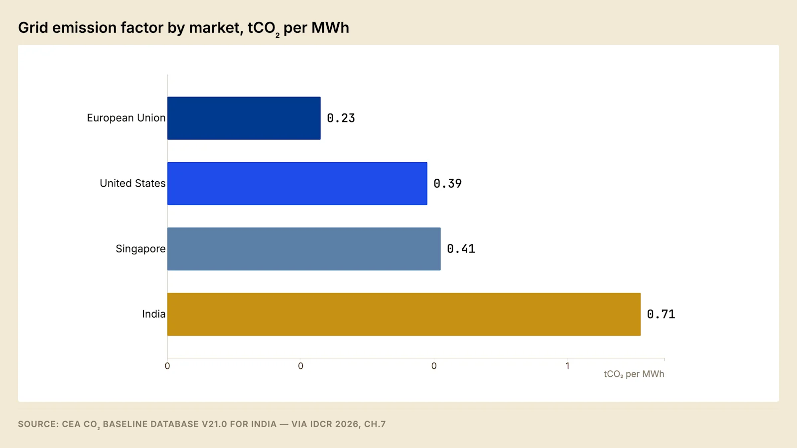
India's factor is high relative to comparable markets, and the gap is the commercial driver behind hourly matching clauses appearing in Indian leases. A tenant running an identical workload on identical hardware reports substantially higher Scope 2 emissions in India than in Europe, and that difference appears in the tenant's own group reporting rather than in the operator's.

2.1 Scope 2 dual reporting under the GHG Protocol #

The accounting standard is the GHG Protocol Corporate Accounting and Reporting Standard with its Scope 2 Guidance, which requires an entity holding any contractual instrument in its supply to report two totals.

In India the location-based factor is the CEA weighted average. A renewable power purchase agreement does not change that total, because it is a property of the grid rather than of the contract, and an operator reporting a reduction against it has made an error a verifier will find. Procurement appears only in the market-based total. Where no residual mix factor is published the grid average is substituted for the unmatched volume, which understates the total to the extent grid-mix attributes are already claimed by others.

An instrument qualifies for the market-based calculation only where it meets the quality criteria in the Guidance.

The temporal criterion is where hourly matching sits: annual matching satisfies it at the coarsest resolution the Guidance contemplates and an hourly clause at the finest.

2.2 The published factor series and version discipline #

CEA revises the weighted average factor annually and the series does not fall in every year, so a base year and a compliance year from different versions produce a change that is partly an artefact.

Sources: CEA CO₂ Baseline Database via Reclimatize, March 2026; India Data Centre Review 2026, Chapter 7.

The table carries two values for the same year from two publications, and they cannot be reconciled from published figures alone, because a value quoted from an earlier version is not withdrawn when a later one supersedes it. The remedy is procedural: name the version, apply it to every year compared, and restate the base year when it changes.

2.3 The boundary of the Scope 2 calculation #

The factor converts purchased grid electricity into emissions and nothing else, so a position assembled from that line alone is incomplete in ways a tenant tests.

The last row produces argument. The operator purchases the electricity and the tenant owns the equipment consuming it, so the same energy appears in the operator's Scope 2 total and in the tenant's upstream accounting. The lease should record which party reports the energy and what data the operator supplies, because a tenant with an hourly commitment cannot compute its position without interval data the operator holds.

Compliance note. Use the same database version for baseline and compliance year calculations. CEA revises the factor annually and inconsistency between versions is a standard verification flag. Where a multi-year commitment is being assessed, state the version explicitly in the methodology note.

2.4 The computation behind the published factor #

An emission factor is a quotient, and every property that separates one published factor from another is a property of how its two terms are bounded. The numerator collects the carbon dioxide released by generation inside a defined electricity system over a defined period. The denominator collects the electricity that the same generation supplied to that system over the same period. The CDM Executive Board's tool supplies the bounding rules, and CEA applies them to Indian plant data.

The last row carries the whole distinction between the three factors set out above. The weighted average admits every plant supplying the system. The operating margin admits the plants whose output would change if demand changed, which excludes generation dispatched irrespective of price. The build margin admits a defined sample of recently commissioned capacity, and the rule defining that sample is a property of the methodology rather than a choice the reporter makes. The arithmetic is identical in all three cases and the population is not, which is why the three cannot be interchanged even though they share a unit.

Two properties of the result follow, and a reporter accepts both rather than adjusting for them. The factor is retrospective, computed from a year that has closed, so a reporting year is always assessed against generation from an earlier period and the lag belongs in the methodology note. The factor is also an annual mean across the whole population, so it carries no information about any individual hour, which is the limitation section 4.1 reaches when an hourly emissions figure is wanted rather than an hourly matching score.

The practical instruction is to treat the factor as a published constant with a version, in the way an engineer treats a code edition. Recomputing it from plant-level data reproduces neither the boundary nor the fuel assumptions the published series uses, and a figure derived that way cannot be reconciled to any other reporter's.

2.5 Average and marginal bases for an emissions calculation #

Two questions about the same consumption take different factors, and the standing of a reported figure depends on which question was asked. The first asks what share of system emissions is attributable to the consumer, which is an allocation and takes an average factor. The second asks how system emissions would differ if that consumption were different, which is a causal statement and takes a marginal factor.

The average basis divides total system emissions across total consumption, so every unit carries the same intensity and the totals of all consumers sum to the system total. That additivity is the reason inventory accounting uses it, because a framework whose parts do not sum to the whole cannot be aggregated into a sector or a national figure.

The marginal basis asks which plants would have run differently. Generation dispatched irrespective of price does not respond to a change in demand and therefore does not enter the calculation, so a marginal factor reflects only the plants sitting at the margin of dispatch in the period concerned. Which of the two factors is the larger follows from the composition of the responding fleet against the system mean rather than from any general rule, and CEA publishes both, so the comparison is drawn from the database rather than assumed.

Three consequences reach practice. A load-shifting claim is a marginal claim, because moving deferrable energy between hours leaves annual consumption unchanged, so an average factor returns no difference and the calculation records nothing at all. A carbon value for shifting exists only against a factor that varies within the year, which is why the flexibility value in Post 10 is built from price rather than from carbon.

An avoided-emissions claim needs a counterfactual as well as a factor. The factor supplies the intensity of the generation that would otherwise have run, and the counterfactual supplies whether it would have run at all. Section 2.7 separates the two accounting frames that question sits between.

The two bases do not mix inside one calculation. A reported total built from average factors and a claimed reduction built from a marginal factor cannot be added, netted or reconciled, and presenting them in adjacent rows of the same table invites precisely that operation.

2.6 The grid boundary and the market boundary #

Two boundaries govern an emissions claim and they are drawn by different authorities. The physical boundary is the extent of the synchronously connected system, inside which generation and load are electrically coupled and a change in one place is met by the system as a whole. The market boundary is the extent of the arrangements inside which an attribute can be created, transferred and retired.

India's transmission system operates as a single synchronous grid, so the physical boundary is national. Energy injected in one region and energy drawn in another are coupled through the same system, which is the reason CEA publishes a factor for the Indian power system rather than one factor for each state.

Deliverability is the row most often left out of a clause. Hourly matching is an accounting operation performed on two contracted quantities, and it returns the same score whether the contracted generator sits inside the same load pocket or at the far end of the system. A clause intending physical coincidence has to say so by naming a delivery point or a region, and the commercial consequence of naming one is the inter-state charge position set out in Post 7.

The boundary also decides what a residual factor would mean. A residual factor is the average intensity of the generation remaining after every claimed attribute has been removed, so constructing one requires a national register of claims. Section 2.1 records that no such factor is published for India, which means the unmatched volume in every Indian market-based total is currently valued at a grid average that still contains attributes other parties have already claimed. The direction of that error is known, its size is not, and the methodology note should say which factor was applied and why.

2.7 Attributional and consequential accounting #

The two questions in section 2.5 belong to two accounting frames that answer different things and are not additive with one another.

The GHG Protocol inventory is attributional. It allocates, so that the totals of every entity in an economy sum to the economy without double counting, and that property is what makes disclosure comparable between operators and aggregable into a sector figure.

A claim about impact is consequential. A statement that a procurement decision reduced emissions asserts that emissions are lower than they would otherwise have been, which requires a counterfactual describing what would have been generated, by which plant, in the absence of that decision.

The two frames are routinely reported in a single document, and the error enters at the junction. An inventory reduction gets presented as an impact, or an impact estimate gets added to an inventory. Neither operation is valid, and the first is the more common because an inventory reduction can occur with no change in system emissions at all. The decomposition in section 3.1 shows the mechanism: procurement that reallocates an existing attribute moves the reporter's market-based total without moving a single unit of generation anywhere.

Additionality is the consequential question stated precisely. An attribute purchased from a plant that would have generated regardless changes the allocation and leaves the system untouched. Whether a procurement decision caused generation to exist is answered by evidence about that plant's investment decision, its route to market and the date of commitment, rather than by anything the instrument itself records. A tenant testing an operator's claim should ask which frame the claim belongs to before asking for the number.

3. The passive improvement #

The grid decarbonises independently of anything a facility does, which produces a reported emissions reduction that requires no action and should not be presented as an achievement.

India's non-fossil share has crossed half of installed capacity and continues to rise, and the published emission factor has declined between recent database versions. A facility with constant consumption and no procurement activity will report lower Scope 2 emissions over time on that basis alone.

The rate of that improvement is the constraint on any commitment made against it. The India Data Centre Review 2026 places Indian grid decarbonisation at roughly one and a half percent a year. A facility relying on grid improvement to meet a 2030 commitment closes a modest fraction of the gap and must procure the remainder, and the arithmetic of how much remains should be done explicitly rather than assumed.

This is also why annual matching claims made against a decarbonising grid convey less than they appear to. A claim that a facility has reduced its emissions is not informative unless it separates the portion attributable to procurement from the portion attributable to the grid.

3.1 Separating the grid effect from the procurement effect #

A reported change in emissions between two years has three components and only one is evidence of action. The decomposition below separates them in a fixed order, because the result depends on the order.

The consumption effect measures growth, so an absolute target set at the start of a ramp is a target to reduce a quantity committed to rise; emissions per unit of IT energy delivered removes it. The grid effect accrues to every consumer in proportion to consumption. The procurement effect exists only in the market-based total, because under the location-based method the sixth step equals the fourth. Diligence asks for the decomposition rather than the movement, since many combinations produce the same change.

4. Annual matching and hourly matching #

Annual matching purchases renewable energy over a year equal in volume to consumption over that year. It makes no claim about when the generation occurred relative to when the consumption occurred.

Hourly matching, expressed as a carbon-free energy score, measures for each hour the proportion of consumption served by clean generation in that same hour, and averages across the year. A facility drawing a flat load and procuring only solar can achieve complete annual matching while a substantial share of its hours are served entirely by the grid, because solar generates for roughly a third of the day and the load continues through the remaining two-thirds.

The mechanism producing the gap is the shape mismatch between generation and load, and it is the same mismatch that drives the banking discussion in Post 7. Annual matching allows the surplus generated at midday to offset the deficit at night arithmetically. Hourly matching does not, because the accounting is performed within each hour and surplus in one hour cannot be carried into another.

The practical consequence for a sourcing lead is that the contract language determines what portfolio must be built. A clause requiring renewable energy equal to consumption "on an annual basis" is satisfied by a solar power purchase agreement. A clause requiring clean energy "in each hour" requires a portfolio combining technologies with complementary profiles, storage, or both. The two clauses differ by a few words and by a large multiple in cost.

4.1 Computing a carbon-free energy score #

The score is computed hour by hour and aggregated once. For each hour the facility has a metered load and a quantity of clean energy delivered under contract, and the matched quantity is the lesser of the two. Delivery in excess of load is surplus, and it is not carried into another hour, which is the entire difference between hourly and annual accounting.

Model assumption — hourly matching across four representative hours

The two aggregations use the same rows and differ by the midday surplus, which one definition credits and the other does not. Four drafting choices change the result and each should be settled in the clause.

The loss convention in the charge stack is set out in Post 7. The residual hours carry a carbon value that is not constant, because the annual factor is a mean while instantaneous intensity moves with the generation mix. India Energy Atlas recorded a national average intensity of 657 gCO₂/kWh at the edition cutoff. An hourly emissions result needs an intensity series at the resolution of the load; where none exists the output is a matching score.

4.2 Data requirements for hourly accounting #

An hourly commitment is a data commitment before it is a procurement one. Six series are required, each with a source, a resolution and a consequence if missing.

Four conditions apply across the six series and none is satisfied by default. Every series must be stamped in one time zone with one convention for whether an interval is labelled by its beginning or its end, because an offset moves the score in one direction and does not average out across a year. The meter must be the revenue meter or a check meter tested against it, since building telemetry will not reconcile to the energy account. The methodology note must state whether a missing interval is interpolated, treated as unmatched or excluded from numerator and denominator. The retention period must match the audit right.

The metering hierarchy behind this is set out in Post 9. Hourly accounting needs depth only to the facility boundary, and a series from every contracted generator, obtained by contract rather than installation.

4.3 The demand-side lever on the score #

The score is a ratio and both of its terms can be moved. Procurement raises the numerator by delivering clean energy into an hour. Load shifting raises the ratio by moving consumption out of hours the portfolio does not serve and into hours where it is already discarding surplus, which raises the matched proportion without contracting an additional megawatt of generation.

The arithmetic follows directly from the matching rule in section 4.1. Because the matched quantity in each hour is the lesser of load and delivery, an hour carrying delivery above load is discarding surplus while an hour carrying load above delivery is unmatched. Moving energy from the second into the first raises the matched total by the smaller of the surplus available and the load moved, and it raises the score twice over, since the unmatched hour loses load while the surplus hour gains matched delivery.

The last constraint bounds the whole lever, because shifting into an hour that is already fully matched adds load and matched delivery in equal measure and leaves the score unchanged. Shifting is therefore worth most in a portfolio with a pronounced midday overshoot and worth least in a portfolio that has already been firmed.

The carbon result and the score result diverge here, and the divergence is the distinction drawn in section 2.5. Shifting improves the score arithmetically wherever surplus exists. Whether it reduces emissions depends on the marginal intensity of the two hours involved, which an annual mean factor cannot express. A clause written on the score credits the first effect; a claim written about emissions requires the second, and the two can point in opposite directions in a system whose evening peak is served differently from its midday.

Shifting also belongs in the portfolio decision rather than in operations, because it lowers the score a given portfolio has to reach and therefore moves the facility down the cost curve. It enters the optimisation in section 5.2 as a decision variable with a cost of its own, which is the value of the service level given up.

5. The cost curve of hourly matching #

The cost of hourly matching is convex. Each additional point of carbon-free energy score costs more than the last, and the curve steepens sharply as the target approaches full coverage.

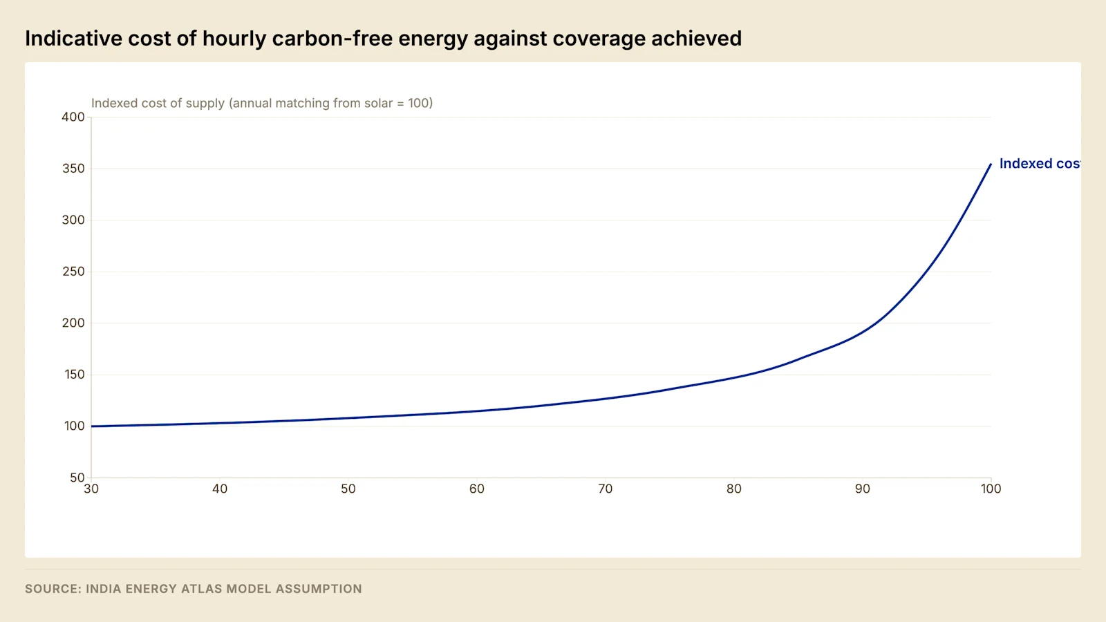
Three regimes are visible in the curve and they have different economics.

The first regime, to roughly the level solar alone delivers, is inexpensive and is achieved by a solar power purchase agreement sized to daytime consumption. The marginal cost is close to the difference between the solar tariff and the grid tariff, which in favourable states is negative.

The second regime is reached by adding wind, whose generation profile is partly complementary to solar both diurnally and seasonally, and by adding modest storage to shift generation across the evening peak. Marginal cost rises but remains within the range a tenant will pay a premium to secure.

The third regime, approaching complete coverage, requires firm clean generation or long-duration storage to cover the hours in which neither solar nor wind is generating. The marginal cost in this regime is multiples of the first, because the assets procured operate at low utilisation and their cost is spread across few hours.

The design implication is that a target should be set at a point on the curve rather than at a round number. A commitment to full hourly coverage is materially more expensive than a commitment to a high but incomplete level, and the difference between them buys very little in reported emissions.

5.1 The residual hours and the utilisation arithmetic #

The convexity has an arithmetic cause that generalises.

The third step is the source of the convexity. A solar plant added to a portfolio that already holds solar delivers most of its output into hours already matched, so the denominator of the fourth step falls while the numerator does not. Storage moves energy between hours rather than creating it and its reach is bounded by its duration, so a four-hour battery reaches the evening and not the pre-dawn hours, which only a longer-duration asset or firm clean generation can cover.

Model assumption — incremental cost of raising the carbon-free energy score

Source: India Energy Atlas model.

The curve is geographic. Its shape depends on the local solar and wind resource, the correlation between them, and the state's banking terms, set out in Post 7.

Field note. Hourly matching cannot be verified without hourly data on both sides of the calculation. That requires interval metering at the facility boundary and generation data at matching resolution from every contracted source. A commitment made without that metering in place is a commitment that cannot be demonstrated, and tenant audit rights under a carbon-free energy clause will require it to be demonstrated.

5.2 Optimisation of a 24/7 portfolio #

The portfolio problem is a constrained optimisation, and stating it in that form makes visible both the data it consumes and the single output that governs a negotiation.

The output worth more than the portfolio itself is the shadow price on the score constraint, which is the cost of the next point of score. That quantity is the cost curve described in this section, and it is the number a sourcing lead needs before signature, because it prices the difference between two draftings of the same clause in the currency the clause is negotiated in.

Four properties of the solution generalise across sites. Correlated resources substitute for one another while uncorrelated resources complement, so a second solar plant in the same resource region adds volume and very little score while a wind site whose profile is uncorrelated adds score per unit of energy delivered. The solution is site-specific, because a generation profile is a property of a resource location, so a portfolio optimised for one delivery point does not transfer to another even at the same target. The constraint binds in a small number of hours, which is the arithmetic reason for the convexity set out in section 5.1, since those hours set the cost of the entire portfolio. And the target itself should be treated as a variable in the negotiation rather than as a constant handed to the analysis, because the shadow price is available before the clause is signed and after signature it is only a bill.

The characteristic failure is optimising on annual volume. A portfolio sized to deliver annual energy equal to annual consumption is the annual matching solution, and it is a feasible point of the hourly problem rather than an optimum of it. Its hourly score is whatever the two shapes happen to produce, and no part of the sizing exercise established what that would be.

Two diligence questions test an optimisation that has already been run. The first asks which hourly series the portfolio was optimised against and over how many years, since a portfolio fitted to a single weather year inherits that year's resource and will underperform in a worse one. The second asks whether the load series was the facility's own metered history or a synthetic profile, because a flat assumed load understates the difficulty of the evening hours at a facility whose load actually rises through them.

5.3 Technologies for the residual hours #

The residual hours have a defining property. Neither solar nor wind is generating, and the deficit persists for longer than a short-duration store can bridge. A resource qualifies for those hours by being dispatchable without regard to weather, or by holding enough stored energy to cross the whole deficit.

The classes divide on one property that decides how a portfolio is sized. An energy-limited resource covers a deficit of bounded length and is exhausted by a longer one, which describes storage and any reservoir with a finite store. An energy-unlimited resource covers a deficit of any length while it remains available, which describes generation with a continuous fuel supply. A portfolio reaching a high score with energy-limited resources alone is exposed to the longest deficit in the record rather than to the average one, so the sizing case is run against the worst period in the series rather than against a mean year.

Firm clean generation is procured as capacity rather than as energy, and the pricing follows from that. Its cost is spread across the few hours it actually serves, so its cost per unit delivered is high while its cost per point of score is the lowest available in that regime. A comparison drawn on landed ₹/kWh alone therefore rejects the only instrument that reaches the third regime, and the correct comparison is the one in section 5.1, against the incremental delivery into hours that are currently unmatched.

The contracting form matters as much as the technology. A firm product is bought as an obligation to deliver a stated quantity in every block, with the counterparty carrying the shaping risk and pricing it, rather than as a share of a named plant's output. That structure transfers the residual-hour problem to a party with a portfolio wide enough to absorb it, and the price difference between a plant-linked contract and a round-the-clock obligation is the market's own estimate of what the residual hours cost.

5.4 Storage as a temporal shifting instrument #

Storage moves energy in time and creates none, so its contribution to a matching score is bounded by three properties, of which the first two are physical.

The attribute question is the part that contracts get wrong. The clean attribute of discharged energy follows the energy that charged the store. A store charged from a contracted renewable plant discharges renewable energy, and that discharge is matched delivery. A store charged from the grid discharges grid energy, and crediting that discharge as clean claims an attribute the grid mix has not surrendered. Separating the two requires metering at the store that records charging energy by source and by interval, which is a contractual requirement before it is a technical one and belongs in the data set in section 4.2 alongside the generator series.

The round-trip loss has a carbon consequence with a determinate sign in each case. Where the store is charged from a contracted clean source, the loss reduces the clean energy available for matching, so the score achieved through the store is lower than the score the same generation would achieve delivered directly into a coincident hour. Where the store is charged from the grid, the loss is additional grid energy drawn and not delivered, and it carries the intensity of the charging hour.

That gives the test for whether a cycle reduces emissions at all. A store charged in a low-intensity hour and discharged in a high-intensity hour reduces emissions where the difference in intensity exceeds the round-trip loss valued at the charging intensity. Where the difference is smaller than that, the cycle raises emissions while still improving a price-based result. The calculation is on the marginal basis described in section 2.5 and it cannot be performed against an annual mean factor at all, which is why a storage carbon claim without an hourly intensity series is an assertion rather than a result.

Two structural choices remain once the store is justified. The first is siting: a store co-located with the generator shifts generation before it is delivered and is charged at the generation bus, while a store at the facility shifts imported energy after delivery and is charged at the meter. The two differ in where losses fall, in their treatment under the charge stack in Post 7, and in whether the charging source can be evidenced at all. The second is reuse of the ride-through asset the facility already holds, which is bounded by the reserve floor and the cycle-ageing conflict set out in Post 6. A battery whose capacity is already committed to backup duty and to the flexibility stack has little left to commit to matching, and the three claims should be reconciled against one asset before any of them is offered to a counterparty.

6. The instruments #

The distinction that matters most is between instruments that deliver energy and instruments that deliver attributes. An unbundled certificate transfers the renewable attribute of generation that occurred somewhere else at some other time. It can satisfy an annual matching clause if the clause permits certificates, and it cannot satisfy an hourly clause under any drafting, because it carries no information about the hour in which the generation occurred.

6.1 The market-based instrument hierarchy #

Instruments rank by the strength of the claim they support, under the GHG Protocol quality criteria and under an hourly clause alike.

An instrument lower in the hierarchy does not substitute for one higher where the clause specifies temporal coincidence: an hourly clause is satisfied by the first four rows, by the fifth only where the certificate records the hour, and by the last two on no drafting. Attribute conveyance is a matter of drafting rather than of physics, and an agreement silent on attributes may leave them with the generator, who is free to sell them separately. A certificate issued in one market cannot be applied to consumption in another.

6.2 Renewable energy certificate issuance and vintage #

A certificate is issued to an accredited renewable generator that has sold its energy without the attribute. Issuance follows verification of injection, and the certificate is extinguished on redemption against an obligation. Purchase discharges nothing; redemption does, and the redemption record is what a verifier examines.

Vintage governs both compliance and any temporal claim. A certificate records the period in which the generation occurred and remains valid for a life fixed by regulation, after which it lapses. That life has been revised, so it is taken from the regulation in force at the transaction date. The recorded period is a month rather than an hour, which is why a certificate cannot evidence hourly coincidence.

The certificate market is residual and thin.

Source: IEX market updates, 2026.

A generator issues certificates only where the unbundled price exceeds what a bundled contract would pay, so supply falls when bundled demand strengthens. An entity planning to meet a shortfall by purchase late in the compliance year is relying on a market that contracts precisely when renewable demand is strong.

Field note. A compliance plan carrying certificates as the balancing item should price them against the current market rather than a historic clearing range, and should specify who bears the cost where the shortfall cannot be covered. In a cost pass-through lease that question is unanswered, because the energy line contemplates energy rather than instruments.

6.3 Carbon Credit Trading Scheme mechanics #

Carbon credits are a separate instrument answering a separate question. The Carbon Credit Trading Scheme's compliance mechanism covers energy-intensive industrial sectors, with intensity targets notified in phases and obligations attaching to installations above a prescribed energy consumption threshold. Data centres are not in the covered list. They are named in reporting on an expected second tranche alongside aviation, ports and railways, and inclusion should be treated as a question of timing rather than of whether: the facilities are large, concentrated, metered and growing rapidly, which makes them administratively tractable in a way diffuse commercial load is not.

Until inclusion, a data centre can participate on the other side of the market. The compliance mechanism is complemented by a voluntary domestic crediting mechanism under which non-covered entities may register eligible emission reduction, removal or avoidance projects for the issuance of tradeable certificates. An operator with a genuinely additional efficiency or procurement intervention has a route to monetise it before obligation arrives.

The compliance mechanism operates on emission intensity at installation level rather than on absolute emissions at entity level. An obligated installation is assigned a target expressed as emissions per unit of output for a target year; one below target earns certificates and one above it acquires certificates to cover the difference, with verification by an accredited agency before issuance.

Sources: International Carbon Action Partnership, India Carbon Credit Trading Scheme, 2026; Indian Carbon Market second tranche reporting, March 2026.

An intensity target does not penalise growth directly, so a sector adding capacity rapidly is not disadvantaged by the form of the obligation, though it is exposed to the level at which the target is set. Intensity requires a denominator, and a data centre has no settled unit of output: candidates include IT energy delivered, computing work delivered and gross floor area, and the choice determines which facilities appear efficient. An operator expecting inclusion should settle the metric, the boundary and the metering behind both, because a target set from a historic baseline uses data already being recorded.

6.4 Contract structures that deliver hourly evidence #

An hourly clause is satisfied by evidence, and that evidence is produced by the generation contract rather than by the lease. Where the generation contract is silent, the operator has promised a tenant something none of its own supply agreements oblige any counterparty to demonstrate, and the gap surfaces at the first audit rather than at signature.

The four structures set out in section 6.1 differ in what evidence they generate as a by-product. Physical delivery through open access produces a settlement record at the load despatch centre, so the hourly evidence exists whether or not anyone contracted for it, and the agreement governing that delivery is set out in Post 7. Group captive produces the same records, subject to the ownership and consumption conditions examined there. An exchange purchase carries the time stamp of the traded block, so the resolution of the evidence is the resolution of the block rather than a matter for drafting. A virtual or financial arrangement produces no delivery record at all, and its evidence is whatever the certificate happens to carry, which returns the instrument to the rank the hierarchy assigns it.

The lease clause should name the same objects the generation contract names. A clause requiring a score without naming the aggregation convention, the residual treatment, the allocation rule, the measurement point, the data the operator will supply and the assurance level obtains a number that neither party can reproduce and that no practitioner can test. Section 4.1 lists the four conventions and section 8.1 the two assurance levels, and a clause that settles all six is shorter than the dispute that follows one that settles none.

Field note. Metering and data obligations are cheap to insert before signature and close to unobtainable afterwards, because a generator carries no commercial reason to accept a new reporting obligation mid-term and every reason to price one. The diligence step that distinguishes a real hourly capability from an intended one is to ask for the data schedule of an executed generation contract rather than the term sheet of a proposed one, and then to ask for one month of the data it produced.

7. Worked calculation #

Model assumption — Scope 2 position, 60 MW IT load facility

The second row of the result is the passive improvement described in section 3, and it occurs with no change to the facility, its consumption or its procurement. Any claim of emissions reduction over a multi-year period should separate this component from the portion attributable to action, and a verifier will ask for that separation.

The calculation also shows why power usage effectiveness carries a carbon consequence disproportionate to its financial one. PUE multiplies IT energy to produce facility energy, so it multiplies emissions on the same basis. The financial sensitivity analysis in Post 1 ranks PUE last among the variables affecting return, and on carbon it ranks considerably higher.

7.1 Emissions intensity of delivered IT energy #

The absolute figure answers the inventory question. An intensity figure answers the comparison question and the target question, and it is obtained by dividing the absolute figure by a denominator of the kind section 10.1 examines. Taking IT energy delivered as the denominator gives a quantity with a closed form.

Model assumption — emissions intensity of delivered IT energy

The last two rows agree because the identity is exact. For a facility drawing all of its energy from the grid, the carbon intensity of delivered IT energy equals the grid emission factor multiplied by power usage effectiveness, and nothing else enters. Two consequences follow. An operator holds exactly two levers over that intensity, one of which is thermal and mechanical and one of which is contractual, and the emission factor is outside its control unless it procures. And any intensity target expressed per unit of IT energy is a target on those two levers alone, which is a narrower commitment than it sounds and a more testable one.

The identity also fixes what a tenant can and cannot ask of an operator. Consumption per unit of computing work delivered is a tenant-side quantity, because it depends on the hardware and the utilisation the tenant chooses, and no operator commitment reaches it.

7.2 Residual emissions at three portfolio states #

An hourly commitment is about the unmatched residual rather than the matched volume, because the residual is the quantity that still carries a factor. The three states below are the anchor points of the cost curve in section 5.1 applied to the reference facility.

Model assumption — residual emissions at three carbon-free energy scores, 60 MW IT load facility

Facility energy and the emission factor from the table above; the three scores are the anchor points of the curve in section 5.1.

The step from the second row to the third removes a modest tonnage, and section 5.1 records what that step costs, which together are the whole argument for setting a target at a point on the curve rather than at a round number.

One caveat governs the reading of the last column. Each residual figure is the unmatched energy valued at the annual average factor, so it is an allocation rather than a measurement of what was emitted during the unmatched hours. Those hours are not average hours, since they concentrate in the pre-dawn and post-sunset periods and in the low-resource months. An emissions figure at hourly resolution requires the intensity series named in section 4.2, and until one is published for India the residual column is the best available approximation and should be labelled as one.

7.3 Implied cost of abatement along the curve #

The cost curve is expressed in ₹ per unit of supply, which is the currency of a procurement decision. Converting it to ₹ per tonne puts it in the currency of a carbon decision and makes it comparable with every other abatement option the operator holds.

Model assumption — implied cost of abatement for two movements along the curve

Incremental cost of supply from section 5.1; factor and facility energy as above.

Three assumptions carry the result and each should be varied before the figure is used. The abated tonnage is valued at the published weighted average, which makes this an attributional calculation of the kind section 2.7 describes; valuing it on the operating margin would answer the causal question instead and would return a different number in a direction the two published factors settle. The incremental cost of supply is applied to the facility's whole consumption, because that is how the underlying curve is expressed, so the figures are blended costs rather than the cost of the marginal unit. And both movements are priced at one point in time, while the curve moves with technology cost and with the charge stack.

The ratio between the two implied costs is the operative output. It says that the same rupee spent in the lower band abates an order of magnitude more carbon than in the upper band, which is the calculation an internal carbon price exists to force into an appraisal, and section 9 sets out how that is done.

8. Disclosed performance #

Reported renewable shares by Indian operators sit well below what an hourly commitment would require. The best publicly disclosed annual renewable share by an Indian operator for FY25 is under half of consumption, and that figure is an annual matching figure rather than an hourly score. The corresponding hourly score would be materially lower.

Facility-level disclosure is absent across the sector, as set out in Post 5 for water and as applies equally to energy and carbon. The consequence for a tenant conducting diligence is that operator claims cannot be verified from public sources, and the verification has to be contractual: interval metering at a defined boundary, generation data from each contracted source at matching resolution, an audit right, and a stated calculation methodology naming the CEA database version.

8.1 Verification and assurance #

Four regimes examine a carbon position against different standards, so evidence prepared for one is rarely sufficient for the next.

The level of assurance is a term of the engagement and belongs in the clause. Limited assurance rests on enquiry and analytical procedure and concludes that nothing has come to the practitioner's attention; reasonable assurance requires substantive testing and is expressed positively. A clause requiring assurance without naming the level obtains the weaker of the two.

Six findings recur, and each has a preventable cause.

• Factor version inconsistency. Base and compliance years from different versions.

• Instruments not retired at the reporting date. Certificates held, not redeemed.

• A double claim on the same attribute. An agreement silent on conveyance.

• The unmatched volume valued inconsistently. An undeclared residual factor.

• Interval data that does not reconcile. Telemetry in place of settlement data.

• An unrestated boundary change. A facility added or removed between years.

Where the boundary, the method or the factor version changes, the base year is restated and both figures disclosed. Without restatement the series measures the accumulated effect of methodology changes.

8.2 The diligence set for a clean energy claim #

Five questions establish whether a stated position can be relied on.

An operator unable to answer the metering question cannot support an hourly commitment whatever the portfolio contracted, which is why it is asked first.

8.3 The audit trail and its order of assembly #

An assurance provider tests a reported figure by tracing it back to a record created for a purpose other than the report, because a record created for the report is evidence of the report rather than of the quantity. The trail is examined from the top down and assembled from the bottom up, and an entity that has never assembled it discovers the missing layer during the engagement.

The practitioner works down from the assertion and stops at the first layer that will not reconcile. Three reconciliations are performed as a matter of course and each fails for a characteristic reason. The meter register against settled energy fails where building telemetry has been substituted for the revenue meter, which section 4.2 identifies as the most common defect in an hourly data set. The contracted volume against registry retirements fails where instruments were purchased and held rather than retired before the reporting date. The aggregated total against the reported figure fails where a facility entered or left the boundary mid-period and the base year was not restated.

Sampling imposes a requirement that is separate from accuracy. A practitioner tests a sample, so the population has to be definable in advance: a list of facilities with their boundaries, a list of instruments with their periods, a list of reporting intervals with their completeness. An entity that cannot produce the population cannot be sampled, and the engagement stops before any testing begins, which is a failure of records management rather than of the carbon position itself.

The level of assurance decides what else is tested. Under limited assurance the practitioner works largely through enquiry and analytical procedure over the aggregation and method layers. Under reasonable assurance the practitioner also tests whether the process reliably produces the figure, which brings four controls into scope: who may edit the aggregation and how that is logged, who authorises the treatment of a missing interval, who approves the methodology note, and how a change of factor version is applied consistently across every period in the comparison.

Two timing rules govern the trail and both are decided long before the engagement. Records have to be retained for longer than the assurance horizon, because a base year restated several years later requires the base year's underlying data rather than its published summary, and the audit right in section 6.4 is worth only as much as the retention period behind it. And the retirement date is the object most often out of sequence, since instruments retired after the reporting date do not cover the period however clearly they identify it.

9. Internal carbon pricing #

An internal carbon price converts a tonne into a rupee so that carbon enters the same appraisal as capital cost and energy cost. Without one, an intervention that reduces emissions and raises cost has nowhere to be compared against an intervention that reduces cost, and the appraisal resolves on cost alone by default rather than by decision.

9.1 Forms of an internal price #

The implicit price is the diagnostic of the three. Section 7.3 computes it for two movements along the cost curve, and the ratio between them is the evidence for setting a target at a point on the curve rather than at a round number. An organisation that computes its implicit price across every intervention it has funded usually finds a wide dispersion, and the dispersion is the recoverable value, because the same budget reallocated toward the cheaper end abates more.

9.2 Application to a data centre decision set #

Four failure modes recur and each is a property of how the price was set rather than of its level. A price below the cheapest abatement available changes no decision, and a price above the most expensive approves every proposal, so the price does work only inside the band its own abatement curve occupies. A shadow price levied on purchased electricity alone systematically favours procurement over efficiency and over any reduction in generator running, because a single scope carries the charge while the others remain free. A price set at group level and not applied by the entity that actually takes the decision is a disclosure rather than a control. And a price applied to a boundary different from the one the target is set on optimises one quantity while the report measures another.

The internal price also has an external reference that does not yet exist in India for this sector. Where the Carbon Credit Trading Scheme extends to data centres, a certificate price becomes observable and the internal price acquires a market anchor and a compliance meaning. Until then the level is a policy choice, and the basis on which it was chosen belongs on the record alongside the number, because a price with no stated basis is revised whenever it becomes inconvenient.

10. Target setting for a colocation operator #

A target is a statement about a future quantity, and four choices settle its content before any number is selected.

10.1 Allocation methods and a growing asset base #

Science-based target methodologies allocate a share of a global carbon budget to an individual entity, and the allocation families divide on whether that share is expressed in absolute or in intensity terms. The distinction decides whether a target is compatible with a build programme.

Absolute contraction requires the entity's emissions to fall at a stated rate irrespective of growth. Applied to an operator whose consumption rises across an occupancy ramp and again with each new building, it requires the procurement effect in section 3.1 to exceed the consumption effect in every single year, so the procurement obligation scales with the build programme rather than with the emissions position. An operator adopting absolute contraction has made a commitment whose cost is set by its own growth rate, and the appropriate response is to size the procurement tranches against the ramp, in the way section 1.2 sizes the compliance obligation.

Intensity convergence requires emissions per unit of output to converge on a sector level, and it permits absolute emissions to rise while intensity falls. It also requires a denominator, and a data centre has no settled unit of output. Section 6.3 sets that problem out for the compliance case, and it returns here in identical form for the target case.

The choice reorders the sector rather than merely rescaling it, which is the reason an operator expecting either a target or an obligation should settle the denominator and begin recording against it before the choice is made externally. The metering to support any of the four is a subset of what an hourly clause already requires under section 4.2.

10.2 Boundary and control in a colocation hall #

The operator purchases the electricity and the tenant owns the equipment consuming it, so the same energy appears twice across the aggregate of corporate inventories. Section 2.3 records the accounting position. The target consequence is separate and is the more contested of the two.

Neither party holds all the levers, so a target set by either is a target over a quantity the other partly determines. Three consequences reach the drafting of a lease. An operator target expressed per unit of IT energy is bounded by the identity in section 7.1, so it is a commitment on efficiency and procurement and on nothing else, however it is worded. A tenant's own efficiency programme, achieved by consolidating onto fewer and better-utilised machines, reduces the operator's absolute emissions while leaving the operator's intensity untouched, so the two target forms respond differently to the same tenant action. And where both parties hold commitments over the same energy, the lease decides which of them may claim the procurement, because an attribute claimed in the operator's market-based total is not available to the tenant, and a tenant with its own commitment needs the attribute conveyed to it as a lease term rather than as an energy term.

Validation and assurance answer different questions and are commonly conflated in marketing material. Validation of a target by a third party confirms that the target was constructed according to a stated methodology, and it says nothing whatever about the reported outcome, which is the subject of section 8.1. A commitment stated without naming the methodology, the base year, the scope coverage and the matching resolution is not testable by either route, and a tenant conducting diligence should record it as a statement of intent and price it accordingly.

Forward look #

Three developments would change the position materially over the next eighteen months.

The first is whether data centres are included in the second tranche of the Carbon Credit Trading Scheme. Inclusion would convert the carbon position from a contractual matter into a compliance one, with intensity targets set at installation level and a reporting obligation attached.

The second is whether hourly matching clauses become standard in Indian leases rather than exceptional. Each such clause requires the metering infrastructure described in section 5, and the aggregate effect would be to create facility-level energy data where none currently exists.

The third is the pace of grid decarbonisation relative to the trajectory in section 3. A faster decline in the emission factor reduces the procurement required to meet any given absolute target, and a slower one increases it. The trajectory is observable annually in the CEA database and should be tracked rather than assumed.

The fourth is whether a residual mix factor or an hourly grid intensity series is published for India. Section 2.6 records that no residual factor exists, so every Indian market-based total currently values its unmatched volume at an average that still carries attributes other parties have claimed. Section 4.1 records that an hourly emissions result cannot be produced without an intensity series at the resolution of the load. Publication of either would change what a clause can require and what a practitioner can test, and would move the subject of an hourly commitment from a matching score toward an emissions figure.

FAQ #

What is the grid emission factor for India? The Central Electricity Authority publishes it annually in its CO₂ Baseline Database. Three factors are published — weighted average, operating margin and build margin — and they answer different questions. Section 2 sets out which to use.

Which carbon obligations apply to an Indian data centre? Renewable purchase obligation under state regulation, any contractual clean energy clause in the lease, and disclosure requirements. They arise from different instruments and are enforced by different bodies, and satisfying one does not satisfy another.

Does the data centre or the distribution licensee carry the RPO? It depends on the procurement structure. Under distribution licensee supply the licensee carries it. Under open access it attaches to the consumer. A facility holding a distribution licence becomes an obligated entity in its own right.

What is the difference between annual and hourly matching? Annual matching purchases renewable energy equal in volume to annual consumption. Hourly matching requires clean generation in the same hour as consumption. A solar-only portfolio can achieve full annual matching while a large share of hours remain grid-served.

Can renewable energy certificates satisfy an hourly matching clause? No. An unbundled certificate carries the renewable attribute of generation that occurred elsewhere at another time, and carries no information about the hour of generation. It cannot establish temporal coincidence under any drafting.

Are data centres covered by the Carbon Credit Trading Scheme? Not currently. The compliance mechanism covers specified energy-intensive industrial sectors. Data centres are named in reporting on an expected second tranche, and can participate through the voluntary crediting mechanism in the meantime.

Sources #

• Electricity Act, 2003, Section 86(1)(e) and state RPO regulations

• Ministry of Power, renewable purchase obligation trajectory notification

• CEA, CO₂ Baseline Database for the Indian Power Sector, Version 21.0, December 2025

• CEA weighted average emission factor series, via Reclimatize, March 2026

• CDM Executive Board, Tool to calculate the emission factor for an electricity system

• GHG Protocol, Corporate Accounting and Reporting Standard and Scope 2 Guidance

• Science Based Targets initiative, corporate target-setting methodology — named at instrument level in section 10; no criterion, rate or threshold from it is stated in this post

• IEX, renewable energy certificate market updates, 2026

• SEBI, Business Responsibility and Sustainability Reporting framework

• International Carbon Action Partnership, India Carbon Credit Trading Scheme, 2026

• Indian Carbon Market, second tranche sector reporting, March 2026

• India Data Centre Review 2026 (v2.3, edition cutoff 28 July 2026), Chapters 7 and 13 — India Energy Atlas

The Scope 2 calculation and the hourly matching cost curve are modelled by India Energy Atlas and are labelled as model assumptions. IDCR 2026 figures are quoted at the locked edition snapshot of 13 July 2026; live Atlas products may carry newer records.

Read the full series — The Indian Data Centre Playbook, twelve parts from unit economics to exit.

Next in the series — Part 9: Operating the Facility. Where designed efficiency is lost in operation, and who captures the value of recovering it.

India Energy Atlas publishes grid carbon intensity, state renewable mix and market price data for India. See energymap.in/pricing.