Cooling Indian Data Centres: Wet Bulb, PUE and the Water Constraint

The short answer. Achievable power usage effectiveness in India is set principally by wet-bulb temperature, which varies enough between Indian cities to produce a material spread in annual energy cost on an identical design. The cooling architecture selected determines both that efficiency and the facility's water draw, and in the markets holding most of India's capacity, water availability under drought conditions is the binding constraint rather than water cost.

This post sets out how cooling architecture determines efficiency and water consumption in Indian conditions, what each architecture costs, and which operational levers change efficiency without capital expenditure. It is written for the design engineer selecting the architecture, the operator accountable for annualised performance, and the tenant negotiating a PUE clause.

Two quantities govern the analysis and are frequently conflated. Power usage effectiveness is total facility power divided by IT power, and it measures the energy overhead of operating the computing equipment. Water usage effectiveness is site water consumption divided by IT energy, and it measures the water cost of rejecting the resulting heat. Improving one commonly worsens the other, which is why they have to be specified together rather than optimised separately.

1. Composition of the non-IT load #

At a design PUE in the range Indian facilities achieve, a substantial fraction of total facility power serves something other than computing equipment. Understanding its composition establishes which interventions can move it.

Model assumption — non-IT load composition at design PUE 1.40

The distribution is the reason cooling receives disproportionate design attention. Every other component of the non-IT load is small enough that halving it would be barely visible in annualised PUE, while the thermal plant is large enough that a modest proportional improvement in it changes the facility's energy bill materially.

1.1 The thermal chain from processor to atmosphere #

Every transfer needs a temperature difference to drive it, and an approach added at any stage is paid for at the compressor, because the chilled water then has to be produced colder or the condenser water accepted hotter. The second and third stages carry the nonlinearity behind variable speed control, since under the fan and pump affinity laws absorbed power varies with the cube of shaft speed, which is also why air cooling has a density ceiling.

1.2 Thermal resistance from junction to coolant #

The chain above is a series of thermal resistances, and each behaves in the same way: the temperature difference across a resistance is that resistance multiplied by the heat passing through it. Junction temperature is therefore the coolant temperature plus the sum of the rises across every resistance between the two, which makes the coolant temperature a facility can deliver a consequence of the device's limit rather than a free choice of the design engineer.

Two consequences follow that a facility engineer meets directly. The first is that the last two rows are where the cooling method changes the answer, because the film coefficient a liquid produces is far above the coefficient an airstream produces at any velocity a hall can tolerate, which is why a device that cannot be cooled by air at a given power can be cooled by a cold plate carrying much warmer fluid. The second is that raising device power raises every temperature difference in the chain in proportion, so a processor generation drawing more power needs a lower total resistance to hold the same junction temperature, and cannot be accommodated by making the room colder.

Thermal throttling is the failure mode at this end of the chain. Where junction temperature approaches the device limit, the processor reduces its clock frequency and its power draw until the balance is restored, so the equipment continues to operate correctly and delivers less work per hour. The hall stays inside its temperature envelope throughout, the cooling plant raises no alarm, and the loss appears only in the tenant's own telemetry. A facility whose commercial product is compute rather than space should therefore treat the inlet temperature distribution described in section 3.4 as a performance measurement rather than as a compliance measurement.

1.3 Sensible heat transport and the temperature difference across a rack #

A fluid stream removes sensible heat in proportion to its mass flow, its specific heat and the temperature difference it gains, so for a given duty the flow required and the temperature difference achieved are inversely related. That single relation governs most of the airside decisions in a hall.

The first row carries the air-cooling ceiling. Rack power rises without the rack's face area rising with it, so the air volume required per unit of face area rises and face velocity rises with it. Pressure drop through the equipment rises with the square of that velocity, the servers' own fans absorb more power and produce more noise, and the floor tile or containment aisle reaches the flow it can physically deliver. The limit quoted in section 3 is the point at which those three effects arrive together, which is why it is expressed as a band rather than as a threshold.

The second row explains why an airside defect presents as a waterside symptom. The temperature difference available across a coil is set by the temperature of the air returning to it, so a hall returning air close to its supply temperature cannot produce the design difference on the water side whatever the control valve does. The plant circulates more water for the same duty, the pumps absorb more power, and the plant reads the narrow difference described in section 3.1 without any waterside component having failed.

Water carries far more heat per unit volume than air at the same temperature difference, which is why a liquid loop moves a hall's duty through pipework of a size that would be unusable as ductwork, and why the pumping power replacing the fan power is a small fraction of it. That comparison is not an efficiency argument by itself, because the compressor may remain in the chain, and section 3.5 sets out the condition under which it leaves.

1.4 The thermal plant's share of the energy bill #

The composition table states the thermal plant's share of the non-IT load as a proportion. Converting it into an annual figure for the reference block gives the quantity against which every efficiency intervention in this post is measured, and it is built entirely from constants set elsewhere in the series.

Model assumption — annual thermal plant energy, 20 MW IT block at design PUE 1.40

Block size, utilisation, design efficiency and the energy price are taken from Post 1, where they are derived.

A proportional improvement in the thermal plant is worth the same proportion of the last row, so a hundredth of the plant's energy is worth several tens of lakhs each year at this block size, and the levers set out in section 7 move considerably more than a hundredth. The same arithmetic bounds the case for capital, because an intervention costing more than the discounted value of the proportion it removes does not pay, which is the calculation applied to immersion in section 3 and to the recovery programme in Post 9.

2. Wet bulb governs #

Dry-bulb temperature determines how much heat must be rejected. Wet-bulb temperature determines how efficiently it can be rejected, because it sets the lowest temperature achievable by evaporative processes and therefore bounds the performance of cooling towers and the availability of free cooling hours.

This distinction is why Indian cooling design cannot be transferred between cities on the basis of latitude or headline temperature. A hot, dry inland location has a high dry bulb and a comparatively low wet bulb, which favours evaporative cooling and delivers many hours in which mechanical cooling can be reduced or avoided. A coastal location at a lower dry bulb but a much higher wet bulb offers neither, because the air is already close to saturation and evaporative cooling has little to work with.

Design should be performed against the coincident wet-bulb condition at the applicable exceedance percentile from the ASHRAE climatic design data for the specific location, and not against an annual average or a figure taken from the nearest large city. The consequence of getting this wrong is a plant that meets its design condition for most of the year and fails it in the weeks when failure is least acceptable.

2.1 Psychrometry of evaporative heat rejection #

Wet-bulb temperature is the temperature a wetted surface reaches in a moving airstream once evaporation and heat transfer come into balance, which makes it the adiabatic saturation temperature of that air and the floor below which no evaporative device can cool water.

The Indian cases are separated by how far the first two sit apart. An inland location before the monsoon presents a high dry bulb with a wide gap to the wet bulb, which is the condition evaporative equipment performs best in. A coastal location holds a narrow gap through the year, which is why the coastal markets show the highest annualised figure.

2.2 Approach, range and cooling tower sizing #

Range is a decision about pumping power rather than about the tower, and approach is where the capital sits, because cold water cannot reach the wet bulb and tower size rises steeply as the approach narrows. A tower selected against an optimistic wet bulb will not make its cold water temperature when the wet bulb is at the design value, and the chiller makes up the difference, which presents as a summer efficiency excursion rather than as a plant failure. The tower approach also governs the waterside economiser, because free cooling is available only when the tower can meet the chilled water supply temperature after the exchanger approach is deducted.

2.3 The design condition and the annualised figure #

ASHRAE climatic design data publishes each of these at several annual exceedance percentiles, so a design condition is a pair of values and a percentile, and quoting one without the other two makes the specification untestable. What happens outside the percentile is a degradation rather than a shutdown, in which the facility spends hours inside the allowable envelope described in section 3.4.

The annualised figure quoted in a lease is produced from that design condition by binning the hours of a reference year by coincident condition, evaluating the plant model in each bin at the load expected there, and weighting by the hours the bin contains. The climate series, the IT load profile and the control sequence are assumptions at that stage, and the last of the three is what separates a design PUE from an operating PUE.

2.4 Dew point, latent load and humidity control #

Computing equipment adds no moisture to a hall. Every gram of water entering the air comes through the envelope, either as the outdoor air supplied to hold the hall at a positive pressure or as infiltration where that pressure is not held, so the latent load is a property of the building and its ventilation rate rather than of the tenant.

The coil is where the latent load turns into an efficiency question. Where the coil surface falls below the dew point of the air entering it, moisture condenses on the fins and part of the coil duty is spent removing water rather than lowering air temperature. Raising the chilled water supply temperature moves the coil surface above the dew point and makes the coil sensible-only, which is a second mechanism behind the largest lever in section 7, distinct from the improvement in chiller efficiency that the same change produces.

Humidity is bounded in both directions by the equipment class described in section 3.4, with a lower bound reflecting electrostatic discharge risk and an upper bound reflecting hygroscopic dust and corrosion on printed circuit assemblies. The characteristic operating defect is a hall in which each air handling unit controls humidity from its own return sensor, so a unit reading low humidity humidifies while a neighbouring unit reading high humidity dehumidifies, and the two consume energy against each other continuously. The remedy is a single hall-level control acting on dew point, with local humidity control at the units disabled rather than merely widened.

Indian coastal halls carry the sharper version of this problem, because the latent component of the outdoor air load in a humid coastal location can exceed its sensible component. Where the fresh air requirement is treated as an addition to the CRAH duty rather than as a separate system, the CRAH units are driven to a low supply temperature by a load that is mostly moisture, the coils condense continuously, and the plant loses both the free cooling hours and the chiller efficiency the higher water temperature would have delivered.

2.5 Components of the design cooling load #

The plant is sized against a coincident condition rather than against the arithmetic sum of each component's individual maximum, because the components peak at different times and a design that adds their separate maxima produces a plant that never operates near its selection point.

The fifth row is the one most often left out of a load schedule, and it has a compounding character the others do not. Absorbed fan power inside the airstream is paid twice, once as electricity drawn by the motor and again as a load the plant must then remove, so a reduction in fan speed returns more than the shaft power saving alone and an oversized fan costs more than its own consumption. The same logic applies to secondary pumps inside a conditioned plant room and to the coolant distribution units described in section 3.5.

Two sizing cases have to be satisfied rather than one. The first is the water-cooled case at the design evaporation wet bulb, which sizes towers, chillers and the condenser water system. The second is the air-cooled fallback case at the design dry bulb, which sizes whatever plant carries the load when water is unavailable and is described in section 5.4. A plant satisfying the first does not necessarily satisfy the second, because the two design conditions do not occur in the same hour and the equipment selected for each is governed by a different ambient property.

3. Cooling architectures #

Six architectures are in use in Indian facilities, and they differ in density ceiling, water consumption, achievable PUE and capital cost.

Source: Mordor Intelligence and operator disclosures, via IDCR 2026, Chapter 8.

Two-thirds of installed Indian capacity uses the architecture with the highest water consumption and the lowest density ceiling. Liquid cooling is the fastest-growing segment of the Indian cooling market from a base below a tenth of installed capacity.

The transition between these architectures is driven by rack density rather than by efficiency. Air cooling reaches a physical limit at approximately 25 to 30 kW per rack, above which the air volume required cannot be delivered through a raised floor or a containment aisle at acceptable fan power. A facility intending to serve accelerated computing has to adopt liquid cooling at some stage regardless of its view on energy efficiency, and the efficiency improvement is a consequence of that decision rather than a reason for it.

The energy case for immersion, considered in isolation, does not support the investment. The annual energy saving from moving a facility from a chilled-water PUE to an immersion PUE is small relative to the capital premium, and the resulting payback extends well beyond any reasonable investment horizon. Immersion and direct-to-chip are purchased to make a high-density rack possible inside a floor plate that could not otherwise accommodate it, and the efficiency improvement appears in the sustainability report rather than in the investment case.

Field note. Direct-to-chip liquid cooling is frequently presented as water-saving. It removes heat from the processor more efficiently and then rejects that heat into a facility water loop that still requires a cooling tower. Unless the heat rejection stage is also changed, site water draw is largely unaffected. The specification should state water usage effectiveness at the facility boundary rather than at the rack.

3.1 The chilled water plant and its distribution defect #

Most Indian capacity above the evaporative threshold is served by chillers, primary and secondary pumps, CRAH units, condenser water pumps and open towers, with a plate heat exchanger for economiser operation and stored chilled water to carry the load through chiller restart. The distribution arrangement carries the plant's most common defect: where secondary flow exceeds primary flow, water bypasses the halls and returns to the chillers close to supply temperature, so the plant reads a narrower temperature difference across the load and starts an additional chiller to remove the same heat, which produces no alarm and surfaces later as a capacity shortfall.

3.2 Chiller part-load performance and the integrated part load value #

The single-number rating used to compare machines across that curve is the integrated part load value, a weighted average of efficiency at several load points, with the weights fixed by the rating standard and derived from an assumed distribution of operating hours. The instrument that defines the rating and its weighting for this class of machine is AHRI Standard 550/590. That distribution describes a commercial building in a temperate climate rather than an Indian data centre, and the standard permits condenser relief at the lower load points, which an Indian summer does not.

Two further properties of the rating limit what it can be used for in a tender. It is established on a test stand at stated conditions rather than in the plant the machine will serve, so the condenser water temperature underlying it is the standard's rather than the site's, and it describes the machine alone rather than the machine with its pumps and tower. A comparison built on the rating therefore ranks compressors, while the quantity a facility pays for is the specific power of the whole plant at the hours it actually runs.

Field note. A chiller tender evaluated on full-load specific power will select the machine that performs worst over the hours the plant actually runs. It should be evaluated against the plant's own hour distribution, at the condenser water temperature the tower delivers at the site design wet bulb.

3.3 Economiser types and changeover logic #

The distinction between the last two rows holds most of the available saving, because a non-integrated economiser operates only when the tower can meet the whole load, while an integrated economiser operates whenever the tower can produce water colder than the chilled water return. Changeover parameters are the ones most often left at factory defaults: the enabling temperature, the deadband that stops the plant cycling as ambient oscillates around the threshold, and the valve transfer that maintains flow to the halls.

Standardised sequences for air handling and central plant control are published in ASHRAE Guideline 36, and the value of referencing a published sequence in a specification is that the behaviour delivered can be tested against a written definition rather than against the commissioning agent's recollection. Three further parameters govern how many hours the economiser actually takes. The first is the minimum dwell time in each mode, which stops a plant transferring on a transient. The second is the position from which changeover is judged, since an enable based on ambient wet bulb anticipates the tower while an enable based on measured condenser water temperature responds to what the tower has achieved. The third is whether the sequence is permitted to run the towers above the speed the mechanical mode would use, which costs tower fan power and buys chiller power at a favourable exchange rate for most of the year.

3.4 Air management, containment and the thermal envelope #

Bypass air leaves the supply plenum and returns to the CRAH without passing through equipment, which wastes fan power and narrows the difference across the coil. Recirculation is the reverse and the more damaging, because the hottest inlet determines whether the facility is meeting its obligation, so supply temperature is depressed until that inlet complies, chiller lift rises, economiser hours fall, and the loss appears in the annual energy figure rather than in any alarm.

What counts as compliance is set by the ASHRAE Thermal Guidelines for Data Processing Environments, which define equipment classes and, for each, a recommended envelope within which manufacturers' reliability data supports continuous operation and a wider allowable envelope within which equipment operates inside warranty for a bounded number of hours. The envelope governing a hall is that of the least capable machine in it, and the allowable envelope is defined with a time weighting, which makes operation inside it for part of the year a designed condition rather than a breach. The lease clause that captures the value states the class, the envelope, the permitted hours and the metering basis.

3.5 Liquid cooling loop architecture #

The two loops are related by the approach across the distribution unit's heat exchanger, and that relationship decides whether the facility loop needs a chiller at all, because the secondary supply temperature the equipment requires sets an upper bound on the facility supply temperature once the approach is deducted. Where the resulting facility temperature is above what a tower or a dry cooler can produce at the site design condition, heat can be rejected without mechanical refrigeration; where it is below, the compressor stays in the chain and the efficiency argument is largely lost.

A direct-to-chip installation does not remove the air plant, because memory, storage, network fabric and power supplies remain air-cooled, and sizing the room air plant on an assumption of complete liquid capture is the most common error in a first deployment, presenting at commissioning as hall temperature rising while the liquid loop operates correctly. Mixed metallurgy in a small-volume secondary loop also produces galvanic corrosion quickly enough to block cold plate microchannels, so material compatibility and fluid chemistry are specification items rather than commissioning items.

Immersion changes the building rather than the plant, because a filled tank loads the floor more heavily per unit area than a populated rack and equipment has to be lifted and drained before it can be worked on. The rear-door heat exchanger is the only liquid arrangement retrofittable into an operating air-cooled hall, and its limit is the airflow the equipment fans can move. Each rejects heat into a facility loop, so the zero in the water column of the architecture table refers to evaporation inside the tank rather than at the plant.

3.6 Airflow delivery and static pressure under a raised floor #

A raised floor is a pressurised plenum, and every perforated tile in it is an orifice discharging from that plenum into the hall. Flow through a tile is set by the static pressure difference across it and by its open area, and the relationship follows a square root, so a proportional change in plenum pressure produces a smaller proportional change in the flow each tile delivers.

The operational consequence is that tile flow cannot be adjusted at one rack without affecting every other rack. Adding tiles increases the total open area presented to the plenum, plenum pressure falls, and flow at every existing tile falls with it. An intervention that appears local is a redistribution of a fixed quantity, and the fixed quantity is set by the fans rather than by the floor.

The last row is the one that surprises an operator, because the racks nearest the air handling unit are the racks most often found hot. Air leaving a unit into the plenum carries velocity pressure that has not yet converted into static pressure, so a tile placed in that region sees a smaller static difference than a tile further along, delivers less flow, and in the extreme case draws hall air downward into the plenum.

Control follows from the same relation. A plant modulating its fans on return air temperature responds to a hall average and cannot detect a maldistribution, whereas a plant modulating on plenum static pressure holds the delivery condition constant and lets the tiles distribute it, which is the arrangement the variable speed lever in section 7 assumes. The measurement set that supports it is a plenum pressure map taken at several points, a hood traverse of tile flow, and an inlet temperature profile at the base, middle and top of a sample of cabinets.

3.7 The slab-on-grade hall and overhead air distribution #

New high-density halls are increasingly built without a raised floor, because the plenum depth required to deliver the air volume grows with rack density until the structural and cost penalty of the void exceeds its value, and because liquid distribution and busway are easier to run overhead than under a floor already congested with cable.

The fan wall changes the redundancy arithmetic. Where a hall is served by discrete air handling units, the loss of one unit removes its whole capacity and the standby unit has to accept the load; where the same duty is delivered by an array of small fans sharing a plenum, the loss of one fan removes a small fraction of capacity and the remaining fans absorb it by raising speed. The array is therefore more tolerant of a single failure and less tolerant of a control failure, since every fan responds to the same signal.

Air distribution on a slab is set at commissioning and is expensive to change, so the flexibility that a raised floor gives away in efficiency it returns in adaptability. The decision follows the tenant profile rather than the technology: a hall let to a single tenant at a known density can be balanced once, while a multi-tenant hall churning racks continuously will spend the life of the building rebalancing a ducted system.

3.8 Fan affinity laws and CRAH selection #

Under the affinity laws, and holding the system curve constant, volume flow varies with shaft speed, developed pressure with the square of speed, and absorbed shaft power with the cube. The consequence is that the largest efficiency gains available in a hall are gains in flow rather than gains in equipment selection.

Model assumption — fan and pump quantities against shaft speed, constant system curve

Derived from the affinity relations. Each column is a fraction of its value at design speed.

The table has two boundaries that a proposal citing it will usually omit. The cube law holds only where the system curve passes through the origin, so a plant controlling to a fixed static pressure setpoint carries a pressure intercept the fan must always develop, and the saving at reduced flow is smaller than the third column suggests. Motor and drive efficiency also fall at the bottom of the speed range, so absorbed electrical power departs from shaft power exactly where the shaft power saving is largest.

Above the density at which airflow rather than duty becomes the binding constraint, the number of units is set by the air volume required and not by the cooling capacity of each unit, and a selection performed on duty alone produces a hall with enough kilowatts of cooling and not enough cubic metres of air. Redundancy is counted in the same currency: an N+1 claim is a claim about airflow available with one unit out of service at the design condition, and it should be evidenced by a test at load rather than by a nameplate sum.

3.9 Chilled water hydraulics and pump selection #

In a closed loop the static lift cancels between the flow and return legs, so pump head is friction alone. Friction rises with the square of flow, which makes pipe sizing an energy decision taken once at design and paid for every hour of the asset's life, since a velocity chosen one increment higher for capital reasons carries a permanently higher pressure gradient.

Pumps in parallel do not add their flows, because the system curve rises as flow increases and the combined operating point sits at the intersection rather than at the arithmetic sum. Staging therefore has to be set from the system curve rather than from nameplate capacity, and a plant staged on a fixed flow threshold will run two pumps where one would have delivered the flow required.

Variable speed pumping only realises the third column of the affinity table where the pressure it holds is measured at the hydraulically most remote circuit. A sensor at the pump discharge holds the head required by the worst case at all times, which converts a variable flow system into a constant pressure one, and pressure-independent control valves are what allow the remote sensor to be trusted, since they hold the flow through each coil irrespective of what the differential pressure elsewhere in the system is doing.

3.10 Primary-secondary against variable primary flow #

The two chilled water distribution arrangements in general use differ in whether flow through the chiller evaporator is held constant, and the choice determines both the parasitic pumping energy and the plant's exposure during a capacity change.

Variable primary flow removes a pump set and the energy it consumes at every hour of the year, and in exchange it makes the bypass valve and the evaporator flow meter critical devices. Adding or removing a machine requires flow to be transferred between evaporators without either machine falling below its minimum flow during the transition, and that sequence is the most demanding in the plant, because it is executed rarely, usually at a rising load, and its failure mode is a chiller trip at the moment additional capacity was being called for.

The selection follows the plant rather than the preference. A plant with few large machines, a wide temperature difference and a stored volume that absorbs the transient tolerates variable primary flow comfortably. A plant with many small machines staging frequently against a narrow difference is exposed, and the exposure is not visible in a design review because the sequence that fails is a transition rather than a steady state.

3.11 Thermal storage and the ride-through interval #

Uninterruptible supply carries the IT load through a loss of grid supply without interruption, and the cooling plant does not recover on the same timescale. Chillers hold an anti-recycle timer, oil and refrigerant conditions have to be re-established, and the motor starting sequence has to complete, so there is an interval during which the hall receives no cooling while continuing to dissipate its full load. At high rack density the thermal mass of the hall itself is small against that load, so inlet temperatures rise within minutes rather than within tens of minutes.

A thermal store in a data centre is a ride-through device rather than a load-shifting device, because load shifting requires hours in which the facility's load is low and a data centre's load profile is close to flat. Where the facility is participating in the flexibility markets described in Post 10, the store becomes a means of moving a share of the cooling load in time without moving the computing load, which is a different proposition and is valued there rather than here.

Two secondary benefits follow from the same vessel. The store absorbs the transient during a chiller stage change, which is what makes variable primary flow tolerable in a plant that would otherwise be exposed, and it reduces the number of compressor starts, which is a maintenance cost rather than an energy cost. Where the chillers sit on generator-backed supply, the store covers the generator start and load acceptance sequence set out in Post 6, and the interval it must cover is that sequence rather than the chiller restart alone.

Field note. A thermal store is frequently installed, commissioned on a fill and a leak test, and never discharged under load. Two defects survive that treatment. The first is a store piped so that discharge enters the return header rather than the supply header, which delivers stored water to the chillers instead of to the halls. The second is a charge flow high enough to destroy stratification, so that the tank holds a uniform temperature part way between charged and discharged and delivers a fraction of its rated capacity. Both are found only by a discharge test with the chillers off and the halls at load.

4. Climate and achievable PUE #

An identical design produces different annualised efficiency in different Indian cities, because the number of hours in which free cooling is available and the efficiency of heat rejection both depend on local climate.

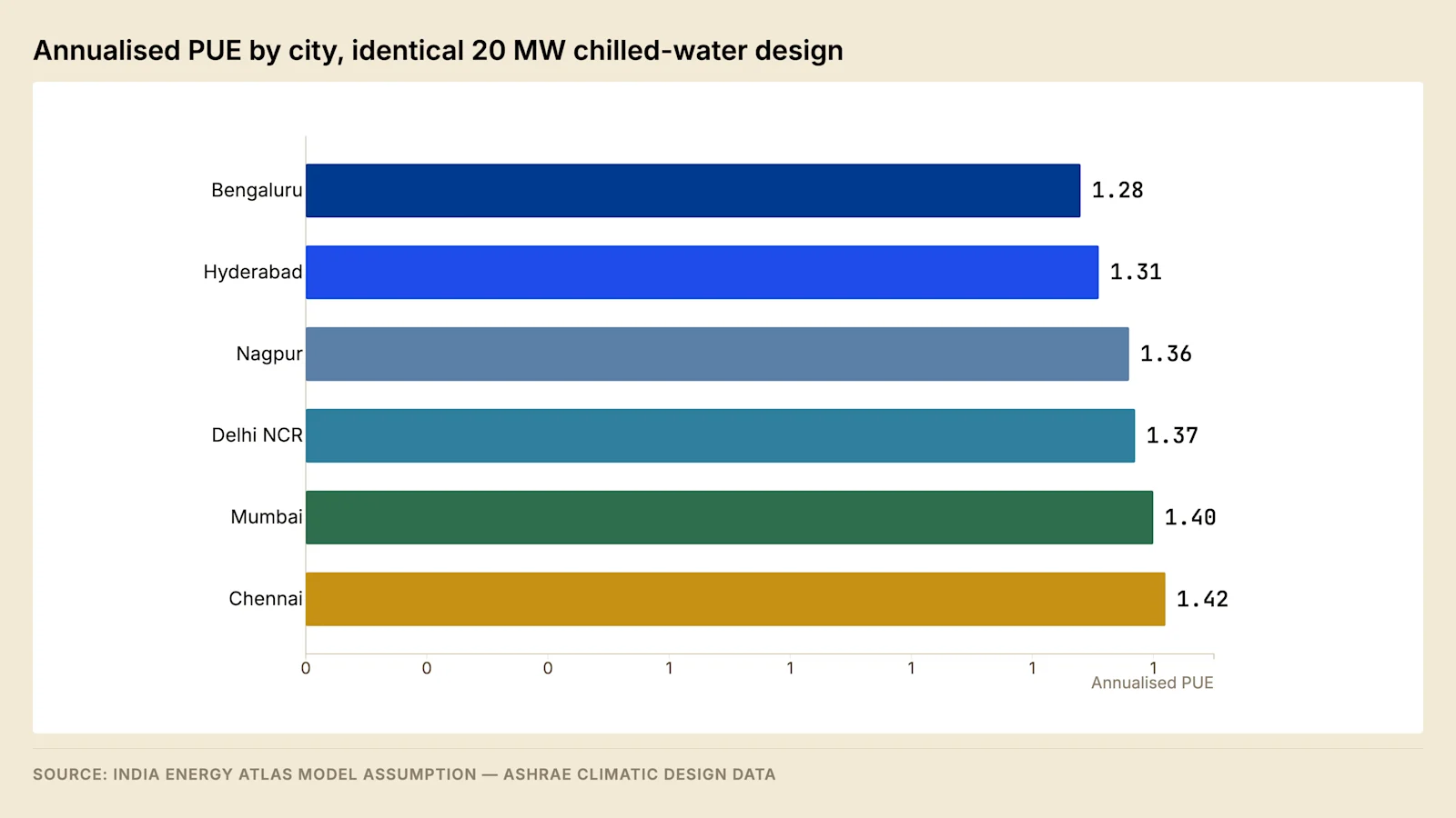
The spread between the best and worst major Indian markets on an identical design is large enough to affect site selection, and it compounds with the state tariff differential set out in Post 2, because the two are not correlated. A market can be favourable on climate and unfavourable on tariff, or the reverse.

The climate penalty is measurable rather than theoretical, and the clearest evidence comes from an operator with unlimited access to capital and to design capability. AWS reports its Hyderabad region as the least efficient of its regions globally, operating well above its own fleet average, notwithstanding custom cooling design and automated plant optimisation. The India Data Centre Review 2026 places the structural penalty imposed by Indian climate at between 0.05 and 0.15 PUE points before any design decision is taken.

The practical consequence is a diligence rule. A design PUE below the range that climate permits, claimed for an air or chilled-water plant in an Indian metropolitan market, requires the measurement category and averaging interval under ISO/IEC 30134-2 to be stated before it is credible. A design-day figure, a partial-load figure and an annualised figure are three different quantities, and only the third has commercial meaning.

4.1 Testing an annualised PUE claim #

The last row connects the two metrics and is omitted most often, because a facility can report a favourable annual PUE by rejecting more heat evaporatively and a favourable WUE by running air-cooled and paying for it in energy, so a specification that caps one without stating the other is an instruction to optimise the uncapped quantity.

Where a design has to be tested against a written efficiency requirement rather than against a commercial commitment, the instrument that states the requirement for this building type is ASHRAE Standard 90.4. It is a design compliance instrument rather than a measurement instrument, so it does not substitute for the operating evidence in section 4.1, and a facility can satisfy it on paper while returning the operating figure described in Post 9.

4.2 Commissioning the thermal plant and the tests that prove capacity #

A thermal plant is a claim about capacity at a condition, and the condition it is designed for is normally not available on the day the plant is handed over. That single fact governs how thermal commissioning differs from the electrical failure-mode testing set out in Post 4, where the failure can be induced at will. The published process instrument for the activity is ASHRAE Standard 202, which defines the commissioning process and the documentation it produces rather than the acceptance criteria for any particular machine.

The capacity test is the one that carries the commercial claim and the one most often left ambiguous. Two remedies exist and they should be chosen before the contract is signed rather than after the test fails. The first is to test at the ambient available and correct the result to the design condition using the manufacturer's certified curves, with the correction method, the instrumentation and the acceptance tolerance agreed in advance. The second is to accept a conditional certificate and hold a retest obligation, with retention, into the season that presents the design condition. The field acceptance procedure for the tower element of that test is published as CTI ATC-105, and naming a procedure in the specification removes the argument about method that otherwise occurs when the measured cold water temperature falls short.

Field note. Thermal commissioning is normally completed with load banks in empty halls, and load banks present a load with a different character from the installed equipment. They draw air at a different rate for the same kilowatt, they present no obstruction map to the plenum, and they can be positioned where the airflow is best rather than where racks will stand. A plant proved on load banks alone has been proved against a load that will never be installed, which is the reason the airflow proof is repeated after the first fit-out and the reason a first tenant frequently reports inlet temperatures the commissioning report does not predict.

4.3 Instrumentation for thermal performance #

Every figure in this post is a measurement or a model of one, and the instrumentation determines which. The measurement categories for the electrical side of a PUE figure are those of ISO/IEC 30134-2, described in Post 9, and the thermal side has no equivalent published category scheme, so the burden of stating what was measured sits with the operator.

The uncertainty in a temperature difference dominates every derived thermal quantity, because the difference is the small remainder of two large numbers and each sensor carries a tolerance of its own. Two sensors individually within specification can produce a difference that is wrong by a substantial fraction of the true value, which is why matched pairs calibrated as a pair are specified for any circuit whose duty will be reported. The same logic bounds what can be inferred: a plant coefficient of performance computed from unmatched sensors is a trend rather than a value, useful for detecting change and unusable for a contractual claim.

Calibration is what separates the two columns above from a set of consistent fictions. An uncalibrated sensor produces a trend that is internally coherent and externally wrong, and it will be believed for as long as it moves in the expected direction. The practices that hold the position are a stated calibration interval with certificates retained, a portable reference carried on the plant walk to check a sample of readings in service, and an alarm on any pair of sensors whose difference becomes physically impossible. Retention and resolution of the resulting data belong to the monitoring boundary described in Post 9.

5. Water #

Heat rejected evaporatively is heat rejected by consuming water, and at facility scale the volumes are large enough to place the facility in competition with municipal and agricultural demand.

Model assumption — water draw, 20 MW IT block on open cooling towers

Switching to air-cooled chillers removes almost all of that draw at a PUE penalty, and the trade can be priced.

Model assumption — the cost of avoiding water

Industrial municipal water in most Indian cities is priced substantially below that figure, and tanker water during scarcity periods generally remains below it. On price alone, water-cooled operation is the correct selection almost everywhere in India.

The decision is not made on price. It is made on availability under the design condition, which is a dry year at peak wet bulb when municipal supply is subject to agricultural and domestic priority. A facility unable to obtain water at any price has an availability problem, and availability problems are not solved by budget. This is why hybrid plants, water-cooled in the base case with full air-cooled fallback capacity installed, have become the default on new coastal Indian builds despite carrying both capital costs.

Sector water consumption follows directly from the architecture distribution in section 3. Indian data centres draw a volume CEEW characterises as comparable to the annual consumption of a city of several million people, and that volume increases substantially by 2030 if the installed base continues to reject heat evaporatively. S&P Global expects the majority of India's data centres to sit in high or extremely high water stress within the decade. The cooling technology transition is the only lever that changes that trajectory.

Source: CEEW 2025 and CEEW with JLL, and S&P Global Sustainable1 2025, via IDCR 2026, Chapter 8. The multiple is derived from the two draw rows.

The projected figure rests on the installed base continuing to reject heat evaporatively in roughly the proportion recorded in the architecture table in section 3. A faster movement down that table changes the sector trajectory without changing the capacity forecast underneath it, which is why the projection is a cooling technology projection rather than a demand projection, and why the third row moves for reasons that have nothing to do with how much computing India installs.

5.1 The water balance and cycles of concentration #

Evaporation cannot be reduced without changing the heat rejection method, because it is the mechanism by which the heat leaves. Drift matters for a reason other than volume, since the droplets carry the dissolved solids and the biological content of the circulating water into the surroundings. Blowdown is the term a water programme operates on, because water leaving as vapour leaves its solids behind.

Moving from low cycles to moderate cycles removes a large share of the makeup requirement, and each further increment removes less and is harder to hold, because the circulating water sits closer to saturation with respect to whichever species precipitates first. The ceiling is set by the least soluble species at the hottest surface in the circuit, which is the chiller condenser tube wall. Operating above the achievable cycles deposits scale on those tubes, which widens the condenser approach and raises compressor lift.

5.2 Makeup water chemistry and source selection #

A treatment programme addresses three processes that occur at once and pull against each other. Scale control holds the scaling species below saturation at the hottest surface, by acid feed to depress alkalinity, by a threshold inhibitor, or by reducing cycles. Corrosion control maintains a protective film on the metal surfaces, which the same acid feed undermines, so the two are balanced rather than optimised separately. Biological control carries a public health obligation, because an evaporative tower is an aerosol generator.

Rainwater harvesting appears in Indian sustainability disclosure as a water strategy, and it delivers volume in the months when plant demand is lowest and nothing in the pre-monsoon months when both the wet bulb and the municipal constraint are most severe. On-site storage is sized in days of makeup at the design condition.

5.3 Heat rejection alternatives #

The closed-circuit fluid cooler is frequently proposed as a water-saving measure and is not one, because it sprays the outside of the closed circuit and evaporates water at approximately the same rate; what it changes is fouling. The hybrid and adiabatic coolers change the shape of water demand rather than its peak, running dry below a switching ambient condition and wet above it, so they retain consumption in the hours when the constraint is most severe.

5.4 The air-cooled fallback and its switchover #

The connection row returns the question to the grid, because air-cooled operation raises total facility power for the same IT load, so where the connection was sized on the water-cooled figure the fallback cannot run at full IT load without exceeding sanctioned demand. The proving row is the one most often unanswerable, because a fallback never transferred to under load is an assumption rather than a capability.

5.5 Adiabatic pre-cooling and the hybrid cooler switching condition #

An adiabatic cooler is a dry cooler with a wetted medium in front of its air inlet. Air drawn through the medium evaporates water and its dry bulb falls toward its wet bulb, with the extent of the fall set by the effectiveness of the medium, so the coil behind it sees cooler entering air and delivers more capacity than the ambient dry bulb would otherwise permit. The device therefore converts a wet-bulb advantage into capacity only in the hours when it is wetted.

The first two rows are the selection question, and a proposal that does not answer it has not been evaluated. A cooler sized dry costs more in coil area and fan power and is indifferent to a water interruption. A cooler sized wet is smaller and cheaper and carries the same exposure the section above describes for the evaporative plant, because the hours in which it depends on water are precisely the hours in which municipal supply is under the most pressure.

The switching condition is the second question. Wetting is enabled on entering air temperature or on the fluid temperature the cooler is failing to achieve against setpoint, and the two produce different water bills for the same capacity. An enable on fluid temperature wets only when the dry capacity has actually run out, which is the parsimonious setting; an enable on ambient wets in anticipation, which is the setting that protects capacity and consumes water on days when the dry coil would have coped.

Water quality on the wetted medium is a maintenance question rather than a chemistry question in most installations, because water evaporating from a pad leaves its dissolved solids on the pad. Scale on a pad reduces its effectiveness and therefore the capacity the device was selected for; scale on a coil surface reduces heat transfer directly. Designs that spray once through to drain avoid the concentration problem and consume more water than a recirculating design for the same duty, so the water figure quoted for an adiabatic cooler should state which arrangement it describes. Every wetted surface in an airstream is an aerosol source, so the control obligations in section 5.7 apply to an adiabatic cooler as they do to a tower.

5.6 Dry cooler selection and the ambient penalty #

A dry cooler rejects heat by sensible transfer from a fluid to air across a finned coil, so the coldest fluid temperature it can produce approaches the ambient dry bulb and can never reach the wet bulb. That single limitation decides where the device is usable in an Indian climate, and it decides it by way of the temperature the load will accept rather than by way of the ambient itself.

The warm-water liquid loop is the case in which the arithmetic works. A cold plate tolerates a supply temperature far above what a CRAH coil requires, so the facility loop temperature that satisfies it sits above the Indian design dry bulb by a workable margin, the dry cooler can produce it, and no compressor appears in the chain for that share of the load. For a conventional chilled water loop the same calculation returns an approach the device cannot deliver, which is why an air-cooled chiller rather than a dry cooler is the water-free option for an air-cooled hall, and why it carries the compressor penalty in section 5.3.

The ambient penalty is therefore not a property of the dry cooler. It is the difference between the temperature the load will accept and the temperature the site's air can deliver, and the liquid cooling transition changes the first of those two rather than the second. This is the mechanism behind the last row of the heat rejection table, and it is the only route in that table that improves the efficiency figure and the water figure at the same time.

5.7 Condenser water treatment and the control of Legionella #

An evaporative tower generates aerosol as a by-product of the process it performs, which places a public health obligation on the operator that is independent of the plant's efficiency and is not discharged by a chemical dosing contract. The instrument that defines the structure of a water management programme for building water systems is ASHRAE Standard 188. The laboratory method for enumerating the organism in a water sample is published as ISO 11731. Neither is cited here for any value it contains, and the series carries no Indian instrument on the point, which is a gap the reader should establish locally rather than assume.

Three physical design decisions carry more of the risk than the dosing regime does. The first is the position of the tower relative to air intakes, occupied areas and the site boundary, because the aerosol travels and the intake draws. The second is the drift eliminator, which is the only device separating the circulating water from the atmosphere and which is inspected in service rather than trusted from a specification. The third is basin design, since a basin that cannot be fully drained and cannot be reached for cleaning will not be cleaned properly whatever the plan says.

Standby plant is the characteristic Indian exposure, because a redundant tower cell, a standby condenser water pump or an isolated branch left full and stagnant at ambient temperature provides the conditions for growth while sitting outside the circulating path the dosing reaches. Rotating duty between redundant items is therefore a control measure as well as a maintenance practice, and a plant operated with a permanent duty and a permanent standby is running an untreated reservoir connected to a treated system.

The treatment programme also interacts with the efficiency programme in both directions. Raising cycles of concentration to save makeup water raises dissolved solids and changes biocide demand, so a chemistry optimised on the scale objective alone increases the biological risk. Biofilm is a strong insulator, so a biological control failure appears first as a widening condenser approach and a rising compressor lift rather than as a health finding, which makes the approach trend described in section 4.3 the earliest operational indicator that the programme has slipped.

6. The disclosure gap #

No major Indian data centre operator publishes facility-level water usage effectiveness. A 2025 investigation by the Earth Journalism Network and Down To Earth found no operator disclosing the metric, and the largest Indian operators publish no water efficiency figure at all. One operator discloses an aggregate recycling volume without a per-facility denominator, which cannot be converted into an efficiency measure.

Source: operator ESG reports and Uptime Institute Global DC Survey 2025, via IDCR 2026, Chapter 8. Indian ranges are estimates; no audited Indian facility-level figure exists.

The disclosure position has a practical consequence for a tenant or an investor. Design WUE figures appear in operator marketing material and are not independently verified, so a WUE figure in a proposal should be treated as design intent rather than as measured performance. The verifiable questions are which cooling architecture is installed, what the makeup water source is, what happens to the design under the drought condition, and whether metering exists at the facility boundary to substantiate a claim at all.

6.1 Metering and diligence on a water claim #

Two boundary decisions change a reported figure without changing the facility. The first is whether the numerator is withdrawal or consumption, which differ by the volume returned as blowdown. The second is whether the figure covers site water alone or includes the water consumed off site in generating the electricity drawn. No facility-level obligation applies in India, and the entity-level regime described in Post 8 binds listed companies alone.

6.2 The elements of a comparable water disclosure #

The absence of Indian disclosure is not the absence of a definition. Water usage effectiveness is defined, with its measurement and reporting requirements, in ISO/IEC 30134-9, which belongs to the same series as the power usage effectiveness standard the industry already quotes. An operator publishing nothing is therefore declining to report against a published definition rather than waiting for one, and a tenant asking for the figure is asking for a standard measurement rather than for a bespoke study.

The denominator carries more of the manipulation risk than the numerator does, because water metering has few defensible variants while IT energy has several, and a ratio can be improved by enlarging its denominator without a litre of water being saved. A disclosure stating the numerator's boundary and leaving the denominator's measurement category unstated has answered the easier half of the question, which is why the two metrics are tested together in section 4.1 rather than separately.

The recycling volume is the specific Indian case worth naming. A recycled or reused volume reported without the total draw and without the facility it belongs to cannot be converted into an efficiency figure, because the reader cannot tell whether it represents a large share of a small draw or a small share of a large one. The disclosure that would settle the question is the makeup meter total, the blowdown meter total, the recycled share of makeup, and the IT energy over the same period, which is four figures a metered facility already holds.

7. Operational levers #

Five interventions move annualised PUE in an operating Indian facility, and they are listed in descending order of effect for a facility already running aisle containment.

Raising chilled water supply temperature. Moving supply temperature upward within the range the installed IT equipment tolerates under ASHRAE allowable conditions increases free cooling and economiser hours and improves chiller coefficient of performance simultaneously. This is the largest single lever and it requires no capital.

Widening the IT inlet temperature band. ASHRAE allowable ranges permit considerably higher inlet temperatures than most Indian halls operate at. The constraint is usually the tenant contract rather than the equipment, so this lever is exercised through lease negotiation.

Variable speed control throughout. Variable frequency drives on chillers, pumps, cooling tower fans and CRAH units, operated under pressure-independent control, convert part-load hours from a penalty into an efficiency gain.

Containment integrity. Hot aisle containment with disciplined management of blanking panels and floor grommets. Recirculation destroys more efficiency than equipment selection recovers, and containment decays continuously as racks are installed and removed.

Staging plant to load. A plant sized for full build-out operating at a fraction of that load during the occupancy ramp is the least efficient condition the facility will experience, and it occurs during the years when the asset can least afford it.

Three of the five require no capital expenditure. They require a controls engineer with a mandate, a commissioning report that is read, and a tenant conversation about inlet temperature bands. The reason they frequently go unexercised is organisational rather than technical, and it is the subject of Post 9.

7.1 Order of exercise and failure modes #

The first row produces incidents, because supply temperature is raised against an average hall temperature, the racks already at the top of the inlet distribution move outside the envelope, and the excursion is attributed to the setpoint change rather than to the recirculation that preceded it. The third row is the check most often omitted, since the test is coil capacity at the new water temperature unit by unit.

7.2 The seasonal recommissioning cycle #

A control sequence tuned once is tuned for the conditions of the week in which the tuning happened. The Indian year presents three thermally distinct regimes to the same plant, the equipment population inside the halls changes continuously, and heat transfer surfaces foul at a rate the design did not assume, so the settings that were correct at handover are correct for a diminishing fraction of the year thereafter. The one-off contractual obligation to return in the opposite season belongs to the construction contract and is treated in Post 9; what follows is the recurring operating cycle that replaces it once the contractor has gone.

The monsoon row carries the cost that surprises an operator, because a plant holding a humidity floor in a hall whose outdoor air is at its most humid will dehumidify continuously and, where a lower limit is enforced, humidify against itself in the manner described in section 2.4. The energy consumed doing so appears in the annual figure as a seasonal excursion with no equipment fault behind it, and the remedy is the control change in that section rather than a plant change.

The cycle is worth what the levers in section 7 are worth, which the arithmetic in section 1.4 sizes, and it costs a small number of engineer-days plus the instrumentation the facility already owns. The reason it is skipped is that its output is a document rather than an incident, and a plant that has not failed produces no requisition. The governance that holds it in place is a standing annual scope in the maintenance contract with named deliverables from the table above, rather than a discretionary optimisation exercise funded from an operating budget when the budget allows.

8. Worked example — the cooling water balance for the reference block #

This example decomposes the daily makeup figure derived in section 5 and tests the operating parameter that moves it. The makeup volume is taken from section 5, and the cycles of concentration is a stated design assumption rather than an observation of Indian practice.

Model assumption — water balance at four cycles of concentration, 20 MW IT block on open towers

Model assumption — makeup at constant evaporation, by cycles of concentration

Evaporation held constant. Arithmetic from the identity in section 5.1.

Evaporation is fixed by the heat being rejected and falls only if the rejection method changes, which is the architecture decision in section 3. Blowdown is set by chemistry, and the second table is what a treatment programme is worth at this facility size, since each step down the cycles column is achieved by a conductivity controller and a side-stream filter rather than by capital plant. The boundary is the makeup analysis.

8.1 Days of on-site water storage at the reference draw #

The water screen in Post 2 asks whether a source is available under the design condition. Where the answer is conditional, the facility buys time rather than certainty, and the quantity of time purchased follows directly from the daily makeup figure above.

Model assumption — on-site storage volume against days of autonomy, 20 MW IT block

Makeup rate taken from section 5, at four cycles of concentration and with the plant running fully evaporative throughout.

The right-hand column is a tank farm rather than a vessel, and its footprint competes with plant yard and future block area on a site whose layout was fixed before the water question was asked. Three qualifications change the number materially, and each of them is a specification item rather than a calculation.

The diligence question is therefore the days of autonomy at the design condition rather than the tank capacity, because the second is a number in a drawing and the first is the quantity the facility actually holds. A satisfactory answer states the volume, the draw it is measured against, whether that draw assumes the fallback is running, and what the store is turned over and treated with while it waits.

8.2 Inputs required for a per-city water figure #

The series brief for this post asks for annualised efficiency and water intensity for the same design across four Indian climate zones. The efficiency half of that comparison exists as the city figures in section 4. The water half does not exist, and it has not been constructed, because no per-city Indian water intensity figure appears in any source this series uses and the value cannot be derived from what the corpus holds.

The response built instead is the decomposition above, which separates the makeup volume into the term fixed by the heat rejected and the term set by chemistry. That decomposition is defensible without any climate series, because the identity holds at every location and only the evaporation term moves between them, and a reader holding a local hourly series and a local makeup analysis can substitute both into the same arithmetic and obtain a figure for that site. The two inputs required are named in the table rather than estimated, and the gap is recorded here so that a later edition can close it with data rather than with an assumption.

The corresponding diligence rule follows from section 6. A per-city Indian water intensity figure encountered in a proposal has been produced from inputs the published record does not contain, so it should be treated as a model output whose assumptions are the deliverable, and the assumptions to ask for are the rows of the table above.

Forward look #

Three developments would change the analysis over the next eighteen months.

The first is whether a national PUE mandate emerges from consultation into notification. A binding efficiency standard would convert the operational levers in section 7 from discretionary improvements into compliance obligations, and would create a reporting requirement where none currently exists.

The second is whether water boards in the stressed markets move from tariff revision to allocation caps. A tariff revision changes the cost of the water-cooled option. An allocation cap removes it, and would force the architecture transition on a timescale set by the regulator rather than by rack density.

The third is the rate at which liquid cooling displaces air in new Indian builds. The transition is currently driven by density requirements at a small number of facilities. If it becomes the default specification for new capacity, the sector water trajectory changes materially and the disclosure gap in section 6 becomes harder to sustain.

FAQ #

What PUE is achievable in an Indian data centre? It depends principally on wet-bulb temperature at the specific location and on the cooling architecture. Indian climate imposes a structural penalty of roughly 0.05 to 0.15 PUE points relative to temperate locations before any design decision is taken.

Why does wet-bulb temperature matter more than dry-bulb temperature? Dry bulb determines how much heat must be rejected. Wet bulb determines how efficiently it can be rejected, because it sets the lower limit of evaporative cooling and therefore the availability of free cooling hours.

How much water does a data centre consume? On open cooling towers at a typical Indian water usage effectiveness, a mid-sized facility draws on the order of 735 cubic metres per day. The derivation, with the facility size and efficiency assumption stated, is set out in section 5.

Is liquid cooling adopted for efficiency or for density? For density. Air cooling reaches a physical limit around 25 to 30 kW per rack. The efficiency improvement from liquid cooling is a consequence of the transition rather than a justification for it, because the energy saving alone does not support the capital premium.

Do Indian operators publish water usage effectiveness? No major Indian operator publishes facility-level WUE. Design figures in marketing material are unverified, so a WUE claim should be treated as design intent unless the measurement category and metering boundary are stated.

What sets the volume of water a cooling tower consumes? Evaporation is fixed by the heat rejected and falls only if the heat rejection method changes. Blowdown is set by the cycles of concentration the makeup chemistry permits, and it is the term an operating water programme addresses. The decomposition for the reference block is in section 8.

Sources #

• ASHRAE, Thermal Guidelines for Data Processing Environments, and climatic design data

• ASHRAE Standard 90.4, Energy Standard for Data Centers

• ASHRAE Standard 202, Commissioning Process for Buildings and Systems

• ASHRAE Guideline 36, High-Performance Sequences of Operation for HVAC Systems

• ASHRAE Standard 188, Legionellosis: Risk Management for Building Water Systems

• ISO 11731, Water quality — enumeration of Legionella

• ISO/IEC 30134-2, Power usage effectiveness measurement categories

• ISO/IEC 30134-9, Water usage effectiveness definition, measurement and reporting

• AHRI Standard 550/590, Performance rating of water-chilling packages using the vapour compression cycle

• CTI ATC-105, Acceptance test code for water cooling towers

• CEEW, India data centre water assessment 2025, via IDCR 2026

• S&P Global Sustainable1, water stress assessment 2025, via IDCR 2026

• Mordor Intelligence, India data centre cooling market, 2026

• Amazon Sustainability Report 2024, regional PUE disclosure, via IDCR 2026

• Down To Earth and Earth Journalism Network, WUE disclosure investigation 2025, via IDCR 2026

• Uptime Institute, Global Data Center Survey 2025

• India Data Centre Review 2026 (v2.3, edition cutoff 28 July 2026), Chapters 8 and 13 — India Energy Atlas

Every engineering standard above is named at instrument level. No clause number, limit value, envelope boundary, rating weight or approach temperature from any of them appears anywhere in this post, because none is held in the series corpus, and where a value would be needed the text states the mechanism and the verification method instead.

The non-IT load composition, the annual thermal plant energy, the affinity-law fractions, the city PUE comparison, the water derivation, the cost of avoiding water, the water balance decomposition and the storage autonomy table are modelled by India Energy Atlas and are labelled as model assumptions. IDCR 2026 figures are quoted at the locked edition snapshot of 13 July 2026; live Atlas products may carry newer records.

Read the full series — The Indian Data Centre Playbook, twelve parts from unit economics to exit.

Next in the series — Part 6: Backup Power Economics. Generator sizing under Indian derating, the emissions regime, and whether storage can displace the diesel plant.

India Energy Atlas builds India's grid intelligence layer. See energymap.in/pricing.