The Unit Economics of an Indian Data Centre: Capex, Revenue and Yield per MW of IT Load

The short answer. A hyperscale-grade Indian colocation facility costs between ₹55 crore and ₹70 crore per MW of IT load to construct, of which the electrical and mechanical power train is the majority. It earns a contracted rent per kW of reserved capacity per month, with energy recovered separately. Stabilised yield on cost falls in the mid-teens, and project return is governed principally by the speed at which contracted capacity fills.

This post sets out the per-MW cost and revenue model for a wholesale colocation data centre in an Indian Tier-1 metropolitan market, and identifies which variables in that model materially affect project return. It is written for the reader who has to construct or interrogate a capital expenditure note: a developer sizing an investment case, a credit fund testing a sponsor's assumptions, or an institutional investor underwriting a stabilised yield.

The model is presented so that it can be rebuilt. Every assumption is stated, every derivation is shown one step per row, and modelled values are separated from sourced values throughout. Modelled figures appear under a "Model assumption" heading and are not attributable to any external source.

Two conditions bound the analysis. It describes a wholesale colocation asset let to a small number of large tenants under long leases, which is the dominant form of new Indian supply. It does not describe retail colocation sold by the rack, enterprise captive facilities, or the GPU-as-a-service businesses that occupy the same buildings, all of which have materially different revenue structures and are addressed in Post 11.

1. The unit of account #

Indian data centre capacity is reported against three different denominators, which are used interchangeably in market commentary and are not convertible without stated assumptions. Establishing which denominator a figure uses is the first step in any comparison, and failing to do so is the most common source of error in Indian data centre analysis.

IT load is the electrical power delivered to computing equipment at the rack. It is the denominator used throughout this series, because it is the quantity a tenant contracts for, the quantity a lease is priced against, and the quantity that determines the size of every other system in the building.

Total facility power is IT load multiplied by power usage effectiveness, plus house and ancillary load. It is larger than IT load by the cooling, distribution and overhead burden, and it is the quantity relevant to the electricity bill and to the grid connection.

Sanctioned load is the contracted demand registered with the distribution licensee, expressed in MVA. It is larger again, because it incorporates power factor and a design margin, and because Indian tariffs levy a demand charge on sanctioned demand whether or not it is drawn.

The final row explains why floor area has been abandoned as a commercial metric. A hall configured for legacy enterprise equipment and a hall configured for accelerated computing occupy comparable floor plates and differ by an order of magnitude in both the power they draw and the revenue they generate, so area no longer carries information about the value of the asset.

Published capacity estimates for the Indian market differ by approximately a factor of three for this reason. Savills India measures colocation IT load. Mordor Intelligence measures total facility power across colocation and enterprise captive facilities, a wider population measured on a wider basis. Neither series is incorrect within its own definition, and neither can be substituted for the other. The same problem affects the 2030 projections, where the India Data Centre Review 2026 and Wood Mackenzie differ principally in their starting baseline and in the proportion of announced capacity each assumes will convert, rather than in their view of the growth rate.

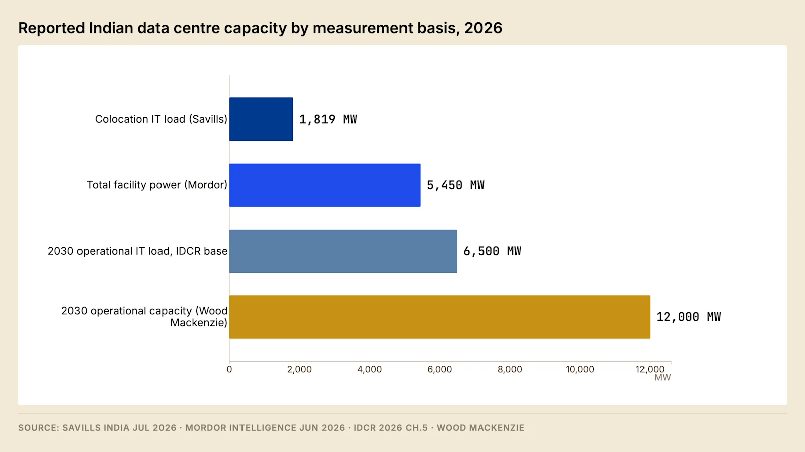
When a broker or vendor presentation arrives, two questions establish whether its capacity figures can be used. The first is which denominator has been applied. The second is whether the capacity described is contracted, commissioned, or merely energised, since these represent three different stages of delivery and are routinely conflated in announcements.

1.1 The five states of capacity #

The second question deserves expansion, because the five states a megawatt can occupy are separated by months of elapsed time and by materially different probabilities of ever reaching revenue.

Announced capacity converts to operating capacity at rates that differ sharply by sponsor class. Tier-one hyperscale facilities have historically converted at a high rate because the sponsor controls its own demand and its own balance sheet. Smaller domestic announcements convert at roughly half that rate, because they are frequently contingent on a tenant that has not signed, a connection that has not been sanctioned, or capital that has not closed.

The practical rule for reading a market forecast is to establish which of the five states its base figure counts, and to apply a conversion assumption to anything counted before energisation. A forecast that counts announcements without stating a conversion rate is a statement about intent rather than about capacity.

1.2 Reconciling published estimates #

Where two credible sources disagree, the reconciliation procedure is mechanical and should be performed before either figure is used.

Establish the denominator, which resolves most of the difference in the Indian market. Establish the population: colocation only, or colocation plus enterprise captive; commissioned only, or commissioned plus under-construction. Establish the vintage, because a figure published in one quarter against a market growing at this rate is materially stale two quarters later. Establish the treatment of partially occupied facilities, which some sources count at full capacity and others at let capacity.

Only after those four are settled can the residual difference be attributed to methodology. In practice the residual is usually small, and the appearance of wide disagreement in Indian data centre reporting is largely an artefact of the four adjustments not being made.

2. Capex composition #

Indian operators do not publish per-MW construction cost, so the composition below is modelled. It is calibrated against published engineering, procurement and construction package tenders and against international cost indices, and it is presented as a model rather than as a market observation.

Model assumption — capex composition, hyperscale-grade Rated-3 equivalent, 20 MW IT block, Tier-1 Indian metro, FY2026 pricing

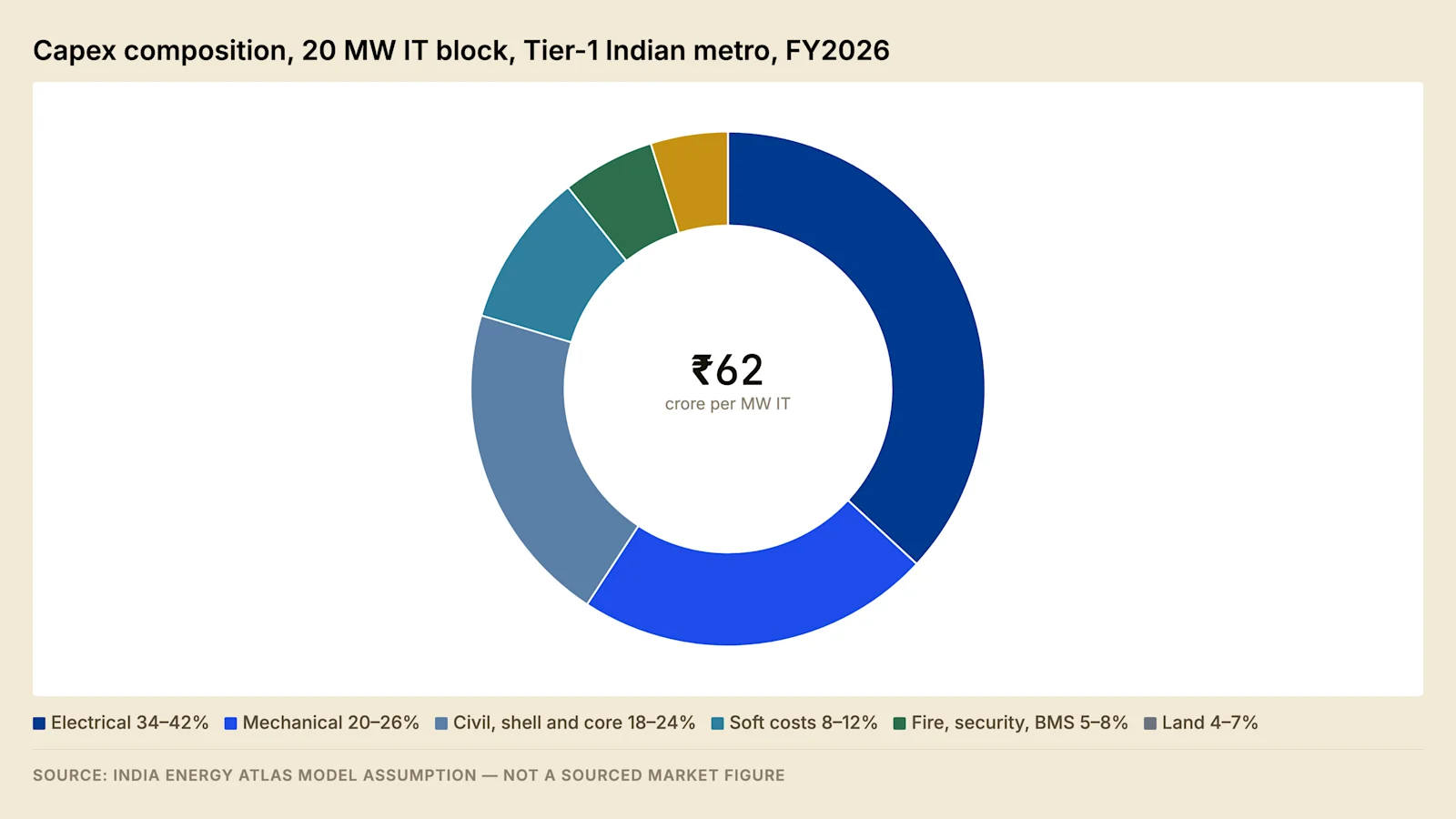
The distribution has a specific consequence for value engineering. The civil package is the element most amenable to cost reduction through design simplification and competitive tendering, and it is a minority of project cost, so savings there are limited in absolute terms. The electrical and mechanical packages are the majority of project cost, and changes to them alter the resilience class of the facility, which in turn determines which tenants can be served and how the asset is valued at exit. Cost reduction in the power train is therefore never purely a cost decision, and is treated separately in Post 4.

The belief that Indian construction cost is materially below international levels holds for the building and for labour, and does not hold for the equipment that carries current. Switchgear, uninterruptible power supply modules, chillers and lithium cells are procured on global supply curves at globally determined prices, and the transformer and switchgear supply chain has not fully normalised since 2022. Expressed in dollars, Indian construction cost per MW sits inside the international range rather than beneath it.

A material portion of the total is attributable to resilience rather than to capacity. Indian grid availability sits below the level a colocation lease commits to, and the difference has to be manufactured on site.

Closing that gap requires uninterruptible power supply capacity with stored energy, standby generation with on-site fuel, and in most cases a second utility feed. The India Data Centre Review 2026 prices this layer per MW, and at prevailing exchange rates it represents between a tenth and a sixth of total project cost. That expenditure buys no additional revenue-generating capacity, and it is not optional for any facility intending to serve institutional tenants.

2.1 Timing of the capital commitment #

The capex table understates the financing consequence because it shows composition rather than timing. The drawdown profile is concentrated, and it is concentrated in the components with the longest procurement lead times.

The third row is where the financing risk concentrates. Long-lead plant is ordered against a specification agreed with the utility, frequently before the connection agreement is executed, for reasons set out in Post 3. A transformer specified for one point of connection has limited value at another, so the capital committed at that stage is substantially irreversible while the outcome it depends on remains outstanding.

This is the structural reason lenders test energisation certainty rather than construction progress, and it is why the diligence pack described in Post 12 is assembled from the connection process rather than from the building programme.

2.2 What moves the capex figure #

Four variables move construction cost per MW materially, and only two are within the developer's control.

Rack density and the resulting cooling architecture. A facility designed for high density carries a cooling capital premium set out in Post 5, and it carries a distribution premium because the busway and secondary distribution are sized for higher current. Both are design decisions.

Redundancy topology. Examined in Post 4. A design decision with consequences for the tenant pool.

Exchange rate and commodity position. The majority of the power train is imported or priced against imported inputs, so the rupee cost of an identical facility moves with the exchange rate and with copper, steel and lithium prices. Not controllable, and it should be carried as a sensitivity rather than assumed constant across a multi-year programme.

Site conditions. Ground conditions, flood mitigation, and the distance to the point of connection. Established during the screening described in Post 2 and largely fixed once the site is selected.

Field note. A capex figure quoted without a stated density, topology and exchange rate is not comparable to any other capex figure. When benchmarking a sponsor's number against a market range, establish those three first; differences of a fifth in headline cost per MW frequently disappear once the specifications are aligned.

2.3 Cost estimate classes and the maturity of the design #

The accuracy of a cost estimate is set by how much of the design exists when the estimate is prepared, and not by the care taken over the arithmetic. Two estimators working from the same issued drawings converge on a similar number. The same estimator working first from a capacity statement and later from a tendered package produces two numbers separated by more than any error either of them contains. Recognising this is what separates a budget from a forecast, and it is the discipline absent from most of the per-MW figures circulating in the Indian market.

AACE International's recommended practice on cost estimate classification sets out the ladder that engineering-led industries use for the purpose. It orders estimates into five classes by the maturity of project definition, running from a screening estimate prepared against a statement of capacity to a check estimate prepared against a substantially complete design. The accuracy range attaching to each class is defined in the practice itself and is not reproduced here, because no Indian data centre calibration of it exists in this series. What transfers is the mechanism: accuracy is bought with design, and there is no other way to buy it.

The document that makes an estimate usable by anyone other than its author is the basis of estimate, and its absence is the first thing to look for. A complete basis of estimate names the deliverables the estimate was priced from, by drawing number and revision. It states the base date at which prices apply. It lists the exclusions. It separates allowances, which cover known scope not yet quantified, from contingency, which covers uncertainty in what has been quantified. It states the escalation, currency and productivity assumptions. It identifies the source of each significant unit rate, distinguishing a tender return from a database rate from a judgement. And it references the risk register against which the contingency was sized.

Two estimates without bases of estimate cannot be compared, because the difference between them may be entirely scope. This is the mechanism behind the observation in the field note above: aligning the specification usually collapses a difference that looked like a difference in cost.

Field note. The characteristic failure is an estimate used outside its class. A screening rate per MW, correct as a screening rate, is carried into a board paper as a budget. The design then develops, scope that was never in the estimate appears, and contingency is drawn to fund it. The overrun is reported as a failure of cost control when its origin is an estimate that was never capable of being a budget, and the evidence for that reading is the date on which each item of the alleged overrun first entered the scope.

The ladder applies to a data centre with one qualification, and it is a consequential one. The building carries two populations of cost that mature at different rates. The shell behaves like commercial construction and can be estimated from area rates at an early stage with tolerable accuracy. The power train behaves like process plant, where cost follows the equipment schedule and the equipment schedule does not exist until the resilience topology is fixed. A single class label applied to the whole estimate therefore conceals a well-defined civil scope sitting alongside an electrical scope that has not yet been designed, and section 2 establishes that the electrical scope is the larger of the two.

The composition table in section 2 sits at the concept-design rung of this ladder. It is a parametric model calibrated against tendered packages, and its intended use is screening, comparison and the interrogation of someone else's number. It does not support a budget.

The diligence question. Ask which deliverables the estimate was priced from, what the base date is, and what the exclusion list contains. A satisfactory answer names drawings by revision, gives a date, and hands over a list. An answer that gives a rate per MW and a range is a screening estimate however it is labelled.

2.4 The engineering, procurement and construction package #

The contract structure determines who prices which risk, and the price responds accordingly. Four delivery models are used on facilities of this scale, and the choice between them is made before the estimate is prepared because it changes what the estimate has to contain.

Standard forms exist for each of the models, of which the FIDIC conditions of contract are one, and the form selected fixes the default allocation of ground conditions, design responsibility and delay. That allocation is what the tender price responds to, so a comparison between two prices let on different forms is a comparison between two different risk positions.

A single commercial arrangement is frequently divided into separate supply and services contracts, with an offshore supply agreement where plant is imported, an onshore supply agreement, and an onshore services agreement covering erection and commissioning. The division follows indirect tax treatment, which is treated with the rest of the tax position in Post 12. Its consequence for the cost model is that the sum of the contract values is the price and the interface between them sits with the owner, unless a wrap agreement or a cross-guarantee binds the counterparties to a single obligation. A comparison between a single lump-sum price and a split-contract structure has to add the cost of the wrap.

Inside a lump sum, the price is assembled from elements that behave differently under negotiation, and knowing which is which determines where a tender can be moved.

The risk allowance row governs the outcome of most tenders. A contractor prices ambiguity. Where the specification leaves a scope boundary open, the tender either carries an allowance sized on the worst available reading or carries a qualification transferring the item back to the owner. Neither outcome is cheaper than defining the scope, and the second is the more expensive of the two, because the item resurfaces during construction as a variation priced without competition.

Owners on facilities of this scale commonly procure the transformers, chillers, uninterruptible power supply modules and switchgear directly and free-issue them to the installing contractor. Three reasons drive the practice. The delivery slot for long-lead plant has to be secured before the installation contract is let, on the programme in section 2.1. The owner wants the manufacturer's warranty and the vendor relationship for the operating life rather than for the defects period alone. And direct procurement makes the largest single element of cost visible instead of embedded in a contractor's price. The cost of the practice is the interface: where free-issue plant arrives late or arrives defective, the installing contractor has a claim for prolongation, and the owner carries a delay it would otherwise have passed down.

The liquidated damages row is where the cost model and the contract meet. Damages are capped, and the cap is set well below the revenue lost when a facility is delivered late, because the revenue lost is the whole of the ramp shifted by the delay, on the mechanism in section 5.1. A contractor's delay exposure is therefore not a hedge against the sponsor's delay exposure, and treating it as one is the same category of error as valuing resilience at the service level credits it avoids, which is examined in Post 4.

2.5 Owner's cost and the boundary of a per-MW figure #

A contract price and a development cost are separated by a body of expenditure that no contractor carries. Comparing a per-MW figure across two projects without establishing which of the two it describes is the most common reason two credible numbers fail to reconcile.

Two of those lines are cross-references rather than new material. The utility connection charge and the attribution of network strengthening are set out in Post 3, and interest during construction sits inside the financing structure in Post 12. Both belong in the cost model regardless, because both are paid before revenue begins.

Three boundaries are in general use, and each of them produces a defensible and different figure for the same building.

The range stated in section 2 sits on the third boundary. It includes land, soft costs, interest during construction and contingency, which is why it sits above figures described as construction cost. A developer quoting the first boundary, a consultant quoting the second and a lender quoting the third are describing one facility, and the bridge between them is a short table whose absence is what makes the three look like a disagreement.

The lines most often missing from a per-MW figure are consistent enough to be checked as a list: the connection charge and any attributed strengthening; interest during construction; commissioning fuel and load bank hire; operator mobilisation ahead of revenue; the fit-out contribution conceded to an anchor tenant; and the cost of a second utility feed where the licensee charges for it separately.

The diligence question. Ask for the bridge from contract value to total development cost, line by line. A satisfactory answer produces it in a table with the owner's costs itemised. An answer that treats the question as pedantry has usually not built the bridge, which means the equity requirement in the model is understated by the amount of it.

2.6 Contingency, its sizing and its drawdown #

Contingency is the fund that covers uncertainty within a defined scope. It is not a fund for scope change, and the distinction determines whether a project that spends its contingency has behaved normally or has quietly become a different project.

The third and fifth rows are the pair that gets confused. A decision to add a chiller, upgrade a topology or extend a hall is a scope change. Funding it from contingency removes the cover the estimate required without recording that the project being funded is no longer the project that was approved. The record that prevents this is a change register in which every draw is classified before it is authorised.

Two of the three understate systematically, and for the same reason: they price the risks on the list. The largest overruns in this asset class arise from items that were on no list, and the most frequent of them is a network requirement emerging from a system study after the budget was set, for which the attribution mechanism is in Post 3.

Contingency has a profile as well as a size, and the profile is the more informative of the two. The fund should decline as risk is retired, and each retirement is an identifiable event.

Field note. The pattern worth looking for in a monthly cost report is a contingency that remains intact through the middle of the programme and is consumed at the end. It indicates one of two conditions, and both present identically in the report. Either contingency was drawn earlier for scope and replaced by re-forecasting elsewhere in the estimate, or commitments have been recognised late so the reported cost has been trailing the committed cost. The evidence that distinguishes them is the commitment register rather than the cost report, and a sponsor unable to produce a commitment register reconciled to the cost report is not measuring the position it is reporting.

The financing consequence is direct. A construction facility sized on total development cost carries the contingency inside the commitment, and the lender's technical adviser certifies the cost to complete at each drawing. Where the certified cost to complete exceeds the undrawn commitment, the sponsor funds the difference before the next drawing is released. Contingency consumed early therefore converts into an equity call long before the works are finished, and the facility mechanics that produce that outcome are in Post 12.

2.7 Escalation over a multi-year programme #

An estimate is priced at a base date. The money is spent over the following years, and the difference between the price on the base date and the price on the date each package is committed is escalation. It is a forecast quantity rather than an uncertain one, it is separate from contingency, and carrying it inside contingency conceals both.

The method is to escalate the spend curve rather than the total. Each package carries its own commitment date, and escalation applies from the base date to that date rather than to completion. Packages committed early carry almost none. Packages left uncommitted until late carry the most. A procurement strategy is therefore also an escalation strategy, and committing a package early converts an escalation exposure into a delivery and cashflow commitment.

Model assumption — escalation applied to the spend curve at a single stated rate. The rate is a placeholder for the reader's own index view; this series establishes no Indian construction escalation rate. Shares are the midpoints of the phase table in section 2.1.

Two features of the result carry into any programme of this shape. The weighted average escalation exposure is close to one year even though the programme runs considerably longer, because the spend is concentrated in the middle rather than at the end. And the escalated total exceeds the base-date estimate by approximately the annual rate itself, which is a serviceable check on any escalation allowance presented for a build of this length.

The second and third rows carry a distinction that is easy to lose. A contract priced in a foreign currency is fixed in that currency and floating in rupees. A contract priced in rupees with a price variation clause is floating in rupees against a published index. A model that treats both as fixed on award understates the exposure, and a model that escalates both understates the value of having ordered early. The exchange rate variable itself is carried as a sensitivity in section 2.2 rather than assumed constant.

Price variation clauses transfer commodity movement to the owner in exchange for a lower tendered price, because a contractor asked to carry a copper position over a two-year delivery prices that position. The choice between a firm price and a variable price is therefore a choice about which party is better placed to carry a commodity exposure, and where the owner intends to hedge the exposure in any event the variable price is usually the cheaper of the two.

2.8 Phasing and the cost per MW #

Phasing splits the capital commitment into blocks that are built and commissioned in sequence. Its effect on cost per MW follows from a division of the capital into three behaviours.

The consequence is arithmetic. Where a fraction of the campus cost is site-wide and the balance divides evenly across the phases, the first phase carries the whole of the site-wide element against a fraction of the capacity. For a campus of equal phases, the first phase indexes at one plus the site-wide share multiplied by one less than the number of phases, and every later phase indexes at one minus the site-wide share.

Model assumption — cost per MW by phase, campus of three equal phases, indexed to the campus average

At a fifth of campus cost sitting in the site-wide element, the first phase costs two-fifths more per MW than the campus average and every later phase costs a fifth less. A developer quoting the campus average while building only the first phase has understated the capital it is about to commit, and a developer quoting the first-phase figure as though it described the asset class has overstated what the market builds for.

Phasing carries costs that offset the exposure it avoids. Switchgear and generator plant are procured in line-ups and sets, so a phased build buys more of both than a single build reaching the same ultimate capacity. Procurement scale is lost, because one order for the whole campus attracts a better price and a better delivery slot than three smaller orders placed a year apart. Mobilisation is repeated, and the later mobilisations occur on a live site, where work is slower, permits are heavier and an error reaches an operating facility. The topology consequences are the more significant of the constraints and are examined in Post 4.

Site-wide infrastructure has to be sized for the ultimate build-out even though the first phase pays for it. A receiving substation, an incoming connection and a water supply sized for the first phase alone converts every later phase into a new connection with its own approval timetable, on the process in Post 3. The saving is real, and it forecloses the campus.

The diligence question. Establish whether a quoted cost per MW describes the phase or the campus, and whether the phase carries its share of the site-wide element. A first-phase figure carrying the whole of the site-wide cost is not comparable with a campus average. A first-phase figure carrying none of it describes a project that cannot proceed to its second phase.

3. The structure of revenue #

Colocation revenue divides into two lines that behave differently, and the margin figures published by Indian operators are not comparable unless the treatment of the second line is known.

The rent line is billed against contracted IT capacity, expressed in rupees per kW per month, and it is charged on reserved capacity rather than consumed capacity. A tenant that has reserved a given quantity of capacity pays for that quantity irrespective of the load actually drawn, which is what makes colocation revenue predictable enough to support long-tenor debt. Escalation is contractual and typically annual.

The energy line is metered and recovered from the tenant. Its treatment varies by contract type, and that variation determines who carries the risk of a tariff revision, who benefits from a procurement improvement, and how the reported margin should be read.

The consequence for reported margins is direct. An operator recovering energy at cost reports a high margin on a small revenue base, because the energy line passes through without contributing to either revenue or profit in the conventional sense. An operator bundling energy into a retail rate reports a lower margin on a larger revenue base. Both may be operating identical facilities at identical profitability in absolute terms, and neither margin figure is meaningful without the contract structure attached to it.

The pass-through arrangement also determines where the benefit of a procurement improvement lands. Where energy is recovered at landed cost, a reduction in the cost of supply reduces the tenant's bill and leaves operator revenue unchanged, so the operator has no financial incentive to pursue it unless the lease provides for sharing. This governs the economics of both efficiency investment and renewable procurement, and is examined in Post 7 and Post 9.

Rent is currently being set under conditions of very low vacancy in the core Indian markets, tighter than the Asia-Pacific regional average and, by the India Data Centre Review 2026's assessment, tighter than any market in the region other than Tokyo. A model constructed on prevailing rents is therefore constructed on the most favourable leasing conditions the market has recorded, which is an argument for testing the downside rather than extrapolating recent escalation.

3.1 The lease terms that move the model #

Rent per kW per month is the headline, and five other lease terms determine what that headline is worth over the life of the asset.

Term and weighted average lease expiry. A wholesale lease runs long enough to support the amortisation profile of the debt against it, and the weighted average expiry across a portfolio is a financing variable rather than a leasing one. A portfolio with a short average expiry is discounted at exit regardless of its current occupancy, for reasons set out in Post 12.

Escalation. A fixed annual escalation is a known quantity. An escalation indexed to a published price index transfers inflation risk to the tenant and introduces basis risk if the index diverges from the operator's actual cost base, which in this asset class is dominated by power rather than by general prices.

Break rights and their conditions. A tenant break exercisable on notice converts a long lease into a short one for valuation purposes. The relevant questions are when the break may be exercised, what notice is required, whether a penalty applies, and whether it is conditional on a performance failure by the operator.

Ramp and take-up provisions. A lease over capacity taken in stages should specify the dates on which each stage becomes payable, and whether rent accrues on reserved capacity from the commitment date or from the take-up date. The difference is a direct transfer of ramp risk between the parties, and it is the single most valuable clause in the agreement for the reasons set out in section 5.

Service level and its remedies. Examined in Post 9. Credits are capped, and the cap is what makes them a poor proxy for the value of resilience.

3.2 Revenue recognition and the reported margin #

Two operators with identical assets and identical cashflows can report materially different revenue and margin depending on how the energy line is treated in their accounts.

Where energy is recovered at cost under a principal arrangement, gross billings including energy appear as revenue and the corresponding cost appears in cost of sales. Where the operator is acting as agent, only the handling margin is recognised. The cash outcome is identical and the reported revenue differs by the entire energy line, which on the model in section 6 is a large proportion of billings.

The consequence for comparison is that revenue multiples across Indian data centre operators are not comparable without establishing the treatment, and EBITDA margin is comparable only after the energy line is stripped from both. The reliable comparison is EBITDA per MW of contracted capacity, because it is invariant to the accounting treatment.

3.3 Pricing a lease from the required return #

A rent is quoted against the market and set against the capital. The market determines whether a rent can be achieved. The capital determines whether achieving it is worth doing. The second calculation runs backwards from the return the sponsor requires, and it is the calculation performed before a developer decides whether to bid for a site at all.

Model assumption — the rent required to return the yield on cost used in section 6

The required return is the input the sponsor controls and the one least often stated. Moving it moves the rent the project needs, and the relationship is close to linear across the range a sponsor would consider.

Model assumption — required rent across a range of required returns, on the section 6 cost and operating assumptions

The base case in section 6 sits between the third and fourth rows. The two ends of the calculation give a rule worth carrying into a negotiation over specification. Each additional ₹1 crore per MW of development cost requires a rent increment to hold the return where it was. On the assumptions above that increment is ₹129 per kW per month, which is the arithmetic behind the position in Post 4 that a topology decision is also a leasing decision.

The calculation is performed per tenancy rather than per building, because the capital attributable to a tenancy is not always the campus average. A tenant requiring a higher resilience class, a dedicated fault domain or a rack density above the design basis draws more capital than the average MW, and the rent returning the required yield on that capital is correspondingly higher. Pricing every tenancy at a campus average transfers value to the tenants with the heaviest specification, and it is the mechanism by which a campus can be fully let at the modelled rent and still fall short of the modelled return.

The boundary. The calculation returns a required rent rather than a market rent. Where the two diverge, the project does not proceed as designed, and four responses are available: a lower development cost, a lower required return, a different resilience class, or a different site. Where the market rent exceeds the required rent, the surplus is development profit, and it is the source of the development spread derived in Post 12.

3.4 Rent review and indexation mechanics #

A lease long enough to amortise the debt against it needs a mechanism to move the rent over its term. Four families of mechanism are in use, and the choice between them determines how much debt the lease will support.

The fourth row is where most institutionally financed leases settle. A cap transfers the tail of inflation back to the operator and a collar removes the downside, and the pair narrows the distribution of the rent. A narrow distribution supports more debt than a wide one with the same expected value, because a lender sizes against the adverse case rather than the central one.

Four questions establish whether an indexation clause will still work in the fifteenth year of a lease. Which index, named by its publisher and by its exact series rather than by a generic description. What happens on rebasing, where the publisher restates the series to a new reference period and the arithmetic of the clause has to survive the restatement. What happens on discontinuance, where the fallback has to name either a successor series or a mechanism for choosing one. And what the reference period is, because an index taken at a single month carries that month's noise into the rent for the following year, while an average over a longer window does not.

Reviews compound on the passing rent rather than on the opening rent, so the base for each review is the rent as previously reviewed. A clause providing for the greater of the indexed rent and the passing rent operates as a ratchet: the rent never falls, and every review starts from the highest level so far reached. The ratchet is worth more than its expected value implies, because it removes the left tail from every future review rather than from one of them.

Model assumption — the rent line under the fixed escalation stated in section 6

The rent doubles a little short of eighteen years at the escalation in the reference model, which is the arithmetic behind the weight a buyer places on remaining lease term. Two otherwise identical assets, one with a long remaining term and one with a short one, are worth different amounts because the second buyer is purchasing a right to re-let at an unknown rent rather than a right to receive a contracted and escalating one. The valuation consequence is derived in Post 12.

The interaction with the operator's own cost base is the part of an indexation clause least often examined. Under a pass-through energy structure the operator's exposed cost is the non-energy stack in section 4, which moves with wages, contracted service rates and insurance rather than with a general consumer price index. A lease indexed to a general index therefore hedges a quantity the operator does not carry, and the residual exposure is the divergence between the two series over the term. Section 4.2 sets out what that divergence does to the margin.

A review not operated on its date does not lapse under most drafting, and three mechanical points determine what the delay costs. Whether time is of the essence, which decides whether the right survives at all. Whether interest runs on the shortfall between the review date and the determination. And whether a memorandum records the reviewed rent, without which the next review has no agreed base. A portfolio carrying several unoperated reviews holds a receivable that does not appear anywhere in the rent roll.

3.5 Churn, re-letting and the effective rent #

Wholesale colocation revenue and retail colocation revenue behave differently over time, and the difference is persistence rather than rate. A wholesale lease is a single long contract with one counterparty, certain until expiry and uncertain at expiry, so its risk is concentrated on a date known years in advance. A retail colocation book is a portfolio of short contracts, each capable of terminating at its own break or expiry, so its revenue depletes continuously and has to be replenished continuously. The measure of the second is churn.

Three churn measures answer different questions and are routinely confused. Logo churn counts customers lost as a proportion of customers held. Revenue churn counts revenue lost as a proportion of revenue billed, and it diverges from logo churn whenever the departing customers are not of average size. Net revenue churn deducts expansion within the retained base, and it can be negative where retained customers grow faster than departing customers leave. A book with high logo churn and negative net revenue churn is growing. A book with low logo churn and positive net revenue churn is shrinking. Only the third measure describes what happens to the revenue line.

Model assumption — the arithmetic of a stated monthly revenue churn rate

The third column is the operative one. At the top of the range the average contract lasts a little over four years, which is shorter than the depreciation life of the plant installed to serve it and far shorter than the amortisation profile of the debt raised against it. A revenue line of that persistence supports materially less leverage than a wholesale rent roll of the same size, which is the financing reason Indian development capital has concentrated on the wholesale form.

The incentives row separates a quoted rent from an achieved rent. An incentive reduces the consideration the tenant pays without reducing the rate the contract states, and market data records rates. In a market where incentives are being given, quoted rents overstate achieved rents by the amortised value of the incentive, and the gap widens as the market softens, because incentives move before headline rates do. Under the accounting standards governing lease income the incentive is spread across the term rather than recognised when it is given, so reported revenue and cash receipts diverge in the early years of a letting.

Effective rent is the measure that reconciles them: the total consideration over the term, net of incentives and of the vacancy assumed before the letting, divided by the term. A buyer capitalises effective rent. A broker report quotes headline rent. The difference is why a rent roll and a market report can describe the same building and disagree without either being wrong.

For the wholesale asset modelled in this post, churn is an event rather than a rate. The equivalent exposure sits at lease expiry and is measured by weighted average lease expiry, for the reasons in section 3.1. The re-let cost is correspondingly lumpy: a wholesale hall vacated at expiry requires the same make-good, reconfiguration and incentive as a retail cabinet, at the scale of a whole hall and on a schedule the operator does not control. A portfolio whose expiries cluster in one year carries that exposure in concentrated form, which is why expiry profile rather than average term is the quantity a buyer examines.

The boundary. Retail colocation revenue per MW, and the rest of the revenue ladder, are treated in Post 11, which is their canonical home. What belongs here is the effect of churn on the revenue line of this model, which appears as a reduction in effective occupancy and an addition to operating cost, and neither is present in the wholesale case modelled in section 6.

3.6 Tenant credit and the receivable #

Contracted revenue is worth no more than the counterparty's ability to pay it. A twenty-year lease against a counterparty with a two-year balance sheet is a two-year lease with an option attached, and the model should treat it as one.

The parent guarantee row is where Indian diligence most often stops short. A hyperscale tenant contracting through a thinly capitalised Indian subsidiary gives the operator recourse to that subsidiary and to nothing else. The parent's credit standing is relevant only to the extent an instrument reaches it, and the strength of the tenant's brand is not an instrument.

The energy line creates a receivable exposure larger than the rent line, and it is specific to the pass-through structure that dominates Indian wholesale colocation. The operator buys the electricity, pays the licensee on the licensee's terms, and bills the tenant afterwards. Both the rent and the recovered energy sit inside the receivable, so the working capital tied up is set by total billings rather than by revenue as an accountant would measure it under an agency treatment.

Model assumption — receivable at the section 6 billing rates, rent and recovered energy combined

Sixty days of billings on the reference block ties up close to a twentieth of development cost. It is funded by equity unless a working capital facility is arranged alongside the term debt, and a model carrying no receivable assumption has understated the equity requirement by that amount. The exposure grows with the energy line rather than with the rent line, so a tariff increase or a hot year raises it without raising revenue.

Revenue is recognised when it is billed and cash arrives later or not at all. The provisioning policy determines when the difference reaches the income statement and the ageing profile determines whether the provision is adequate. Two operators with identical collection performance can report different EBITDA for a period by provisioning against different triggers, which is a second reason, alongside the energy treatment in section 3.2, that reported margins across Indian operators are not directly comparable.

A written-off receivable costs more than the revenue it represented. The rent is lost. The energy already purchased and delivered is lost at its landed cost rather than at the operator's margin on it. And the capacity has been occupied for the period without earning, so the opportunity to let it to a paying tenant has also been lost. Under the pass-through structure the second of the three is the largest, because the operator has been funding the tenant's electricity.

The remedies available to a colocation operator are weaker than the lease implies. Suspension of supply to a live tenant is available under most drafting and is rarely exercised, because the operator's obligations to other tenants on shared infrastructure, the risk to equipment on an uncontrolled shutdown, and the reputational consequence in a market with few operators all argue against it. A lien over tenant equipment is slow to enforce and the equipment is worth little to anyone other than its owner. The instruments that work are the ones taken before occupation.

The diligence question. Four figures describe the credit quality of a rent roll: the ageing profile of receivables, the concentration of billings in the largest counterparty, deposit and guarantee cover expressed in months of billings, and the provision as a proportion of receivables with its trend over recent periods. A rent roll presented without them is a list of contracts rather than a description of income.

4. The operating cost structure #

Operating cost divides into energy and non-energy components, and only the second is genuinely within the operator's control on a wholesale lease.

Energy consumption is determined by IT load, by the utilisation of that load, and by power usage effectiveness. Because PUE is a multiplier on IT energy, a facility operating at a higher PUE consumes proportionally more total energy for the same delivered computing capacity, and in a bundled contract that difference falls directly to the operator's margin.

Non-energy operating cost comprises planned and corrective maintenance across the electrical and mechanical plant, technical and security staffing on a continuous shift basis, insurance, property tax, spares inventory, and the software and licensing associated with monitoring. It scales with installed capacity rather than with occupancy, which means it is incurred in full from commissioning while revenue accrues only as capacity is let. This asymmetry is the principal reason early-year returns are weak, and it is quantified in section 6.

Model assumption — non-energy operating cost, 20 MW IT block at stabilised occupancy

4.1 The behaviour of each operating cost line #

The table above states a stabilised figure per MW. What it does not state is how each line behaves when occupancy, commissioned capacity or plant age changes, and that behaviour determines the cost in every year other than the stabilised one.

Two lines in the table move with occupancy and neither is large. The shift establishment behaves as it does because the control room has to be covered continuously whether the halls are full or empty, and its composition is set out in Post 9. This is the mechanism behind the asymmetry described in section 5, stated line by line rather than in aggregate.

Model assumption — non-energy operating cost through the ramp, per MW of commissioned and of let capacity

In the first year of operation the non-energy operating cost carried by each MW earning revenue is close to three times its stabilised level. Nothing about the facility has changed between the first row and the last; the denominator has.

A second behaviour appears over a longer horizon. Maintenance cost on rotating and switching plant rises with age, and it rises in steps rather than smoothly, because the manufacturer's schedule specifies major interventions at intervals — a generator top-end overhaul, a chiller compressor rebuild, a battery replacement, a switchgear refurbishment. Each is a capital-scale expenditure arriving inside an operating budget. A model holding operating cost flat in real terms across a twenty-year horizon has omitted them, and the omission concentrates in the years while the debt is still amortising. Lifecycle reserves are the usual response, and their treatment inside a financing is in Post 12.

4.2 Divergence between rent escalation and cost escalation #

Rent escalates under the lease. Cost escalates under the market. The two rates are set by different mechanisms and there is no reason for them to agree, so the margin moves across the life of a lease in the direction determined by which of them is larger.

Model assumption — the reference block after ten years of escalation, rent escalating at the contractual rate in section 6 and the retained energy margin held flat

A cost base escalating four points above the rent removes about nine-tenths of a point of compound earnings growth over a decade. The effect compounds a second time in the exit value, because a buyer capitalises the earnings of the year in which it buys rather than the earnings of the year the lease was signed. The clause fixing rent escalation and the procurement decisions setting cost escalation are therefore the same decision approached from two sides, and they are usually taken by different people at different times.

Two structural features of this asset class make the divergence more likely than in general commercial property. The exposed cost base is technical rather than general: contracted maintenance on imported plant, insurance on a reinstatement value that moves with equipment prices and with the exchange rate, and a skilled technical establishment competing in a labour market with more demand than supply. And the rent side is frequently fixed at a percentage negotiated years earlier against a different expectation of inflation. The hedge available is on the cost side rather than on the rent side, through long-tenor maintenance agreements with stated escalation and multi-year insurance placements, both of which are cheaper to obtain before the facility has a claims history than after.

4.3 Diligence on an operating cost budget #

An operating cost budget is presented as a figure per MW per year, which is the form in which it is least testable. Seven questions convert it into something that can be checked.

The first row does most of the work. A budget stated against let capacity ramps alongside revenue and produces a model showing a profit in the first year, which is the reconstruction error identified in section 6.2. The remaining six establish how much of the number is a contract and how much is an opinion, which is the distinction a lender's technical adviser is employed to draw.

5. The occupancy ramp #

A commissioned data centre does not let instantaneously. Capacity fills over a period governed by tenant demand, by the sequencing of tenant equipment installation, and by the phasing of the building itself, and the resulting curve is the single most important determinant of project return.

The mechanism is straightforward. Non-energy operating cost and debt service are incurred against the full commissioned capacity from the date of commissioning. Rent accrues only against let capacity. Until occupancy reaches a level at which rent covers both, the asset produces a return below its cost of capital, and every month spent in that condition is a permanent reduction in the internal rate of return that cannot be recovered by later performance.

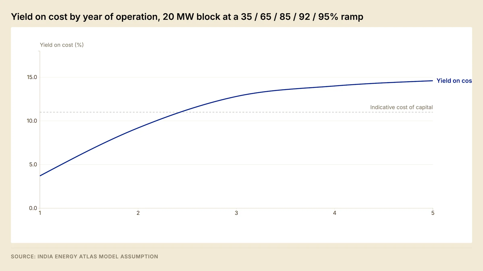
The practical consequences follow directly. Anchor tenancy is secured before construction commences, because a signed anchor lease compresses the ramp and materially improves the financing terms available. Conceding on headline rent to secure an anchor is generally the correct trade, because the reduction in rent applies to a portion of the capacity while the improvement in the ramp applies to the whole asset. Hyperscale tenants accounted for the substantial majority of Indian absorption in the first half of 2026, which is why development activity is concentrated on the small number of markets those tenants will consider.

Phasing the building is the second mechanism available. Constructing and commissioning in blocks rather than as a single monolithic hall reduces the capital exposed during the weakest part of the ramp, at the cost of some duplication in switchgear and a loss of scale economy in procurement. That trade is examined in Post 4.

5.1 The asymmetry of ramp risk #

A delay to the ramp is not recovered by a subsequent acceleration, and the reason is arithmetic rather than commercial.

Return is a function of the timing of cashflows as well as their magnitude. A year of earnings foregone at the start of an asset's life is discounted least and is therefore worth most, while a year of earnings added at the end is discounted most and is worth least. An asset that reaches stabilisation a year late does not recover that year by operating a year longer, because the two years are not equivalent in present value terms.

This asymmetry is why the sensitivity in section 7 places occupancy timing above rent. It also explains a pattern that appears counter-intuitive in the market: operators conceding materially on headline rent to secure an anchor lease before construction. The rent concession applies to a portion of the capacity for the term of that lease. The ramp improvement applies to the whole asset at the point in its life where cashflow timing is most valuable.

5.2 Testing a sponsor's ramp assumption #

A ramp assumption in a sponsor's model is the assumption most worth interrogating and the one least often evidenced. Four questions establish whether it is credible.

What is contracted at financial close, and on what terms? Capacity subject to a signed lease with a defined take-up date is evidence. Capacity subject to a letter of intent, a memorandum of understanding or a term sheet is not, and should be treated as speculative until the conditions in it are satisfied.

What is the take-up profile within the contracted capacity? A tenant that has leased capacity in stages will occupy it in stages, and the revenue profile follows the take-up dates rather than the lease date.

What comparable ramps has this sponsor achieved? Historical performance on previous facilities in the same market is the strongest available evidence, and its absence in a first-time developer is itself a finding.

What happens to the ramp if energisation slips? The ramp cannot begin before the facility is energised, so a connection delay shifts the entire curve rather than compressing it. A model that shows a delay to energisation without a corresponding shift to the ramp has not modelled the delay.

5.3 Phase size against the absorption rate #

Phasing is usually discussed as a capital decision. It is also a leasing decision, because the size of a phase determines how much commissioned capacity stands unlet while it fills.

Where a phase fills at a steady absorption rate, the capacity standing unlet averages half the phase across the fill period. Over a campus built in equal phases, the total exposure measured in MW-years is the campus capacity multiplied by the phase size and divided by twice the absorption rate. The exposure is proportional to the phase size, so halving the phase halves it, irrespective of how many phases the campus is eventually divided into.

Model assumption — unlet capacity exposure on a 20 MW campus absorbing at 10 MW a year

Each MW-year of unlet capacity forgoes the rent and the retained energy margin on that MW while incurring the operating cost against it in full. At the reference rates, the exposure avoided by moving from a single phase to four is worth approximately ₹168 crore of foregone revenue, against which the duplicated switchgear, the lost procurement scale and the repeated mobilisations described in section 2.8 have to be set.

Two conditions bound the calculation, and both fail in identifiable circumstances. It assumes later phases can be commissioned on demand, which requires the site-wide infrastructure to have been built for the ultimate capacity and the connection to have been sanctioned for it, on the process in Post 3. And it assumes the absorption rate is independent of the capacity available, which fails wherever a tenant requires a commitment to capacity beyond the current phase before signing anything. That failure is common with hyperscale requirements, and it is the reason a phased campus still needs a connection sanctioned for the whole build-out even though the buildings arrive one at a time.

6. Worked example #

Every value below is a model assumption. Substituting actual deal terms preserves the structure of the calculation.

Model assumptions — 20 MW wholesale block, Tier-1 Indian metro

Per-MW annual result at stabilised occupancy

The same result expressed as a margin depends entirely on which revenue base is used as the denominator. Measured against total billings including recovered energy, the margin is approximately half. Measured against the rent line alone, it approaches ninety percent. Both describe the identical asset, and neither is informative without the basis stated.

6.1 From EBITDA to equity return #

Yield on cost measures the asset. Equity return measures the investment, and the two diverge because of leverage, tax and the timing effects described in section 5.

Model assumption — equity position on the same block

The coverage ratio at stabilisation is comfortable. The ratio during the ramp is not, and it is the binding constraint on how much debt the asset can carry at financial close. A facility at first-year occupancy produces EBITDA well below its debt service, which is why construction facilities are structured with an interest reserve, a capitalised interest period, or sponsor support until a coverage test is met.

The equity return therefore depends on three things beyond the asset's operating performance: how much debt the ramp will support, how long the sponsor must fund the shortfall, and whether the facility can be refinanced at stabilisation on terms that reflect its de-risked profile. Post 12 sets out that refinancing and the exit that follows it.

6.2 Rebuilding this model #

The model can be reconstructed from the assumptions stated in this post, and doing so is the recommended way to use it. The sequence is:

1. Set contracted IT load and the capex rate per MW to obtain development cost.

2. Apply the rent rate to contracted capacity to obtain the rent line, with escalation applied annually from the take-up date rather than the lease date.

3. Derive energy consumed from IT load, utilisation and PUE; apply the landed energy rate to obtain the energy line; apply the handling margin to obtain retained energy income.

4. Apply the non-energy operating cost per MW, held flat against commissioned capacity rather than let capacity.

5. Apply the occupancy ramp to the rent line and to energy consumption, and not to operating cost.

6. Compute EBITDA by year, then yield on cost against development cost.

7. Layer debt service and test coverage in each year, not only at stabilisation.

Step four is where most reconstructions go wrong. Operating cost scales with the capacity commissioned, not with the capacity let, and a model that ramps operating cost alongside revenue understates the early-year loss and overstates the project return.

6.3 The ramp years and the coverage profile #

The sequence above is performed below, so the result can be checked rather than described. Rent is held at its opening level so that the occupancy effect is visible on its own; applying the contractual escalation raises every year after the first and is treated separately in section 4.2.

Model assumption — the reference block through the ramp, 20 MW, rent held at its opening level

Three readings follow from the table. The first year produces earnings well below debt service, and on this profile the shortfall is close to ₹54 crore, which is about an eighth of the sponsor's equity and falls due after that equity has already been spent on construction. Coverage passes unity during the second year and reaches its stabilised level only when the ramp completes, so a covenant tested from the first payment date would be breached on a facility performing exactly to plan. And the operating cost column does not move at all, which is the asymmetry described in section 5 expressed as a column of identical figures.

The funding response is structural rather than operational, and three forms are in use: an interest reserve funded at financial close, a period during which interest is capitalised rather than paid in cash, and sponsor support until a coverage test is satisfied. Which of the three applies determines when the sponsor's money is at risk and for how long, and the facility mechanics that implement them are set out in Post 12.

The same profile expressed as a yield on cost is the curve in the figure at section 5. Reading the two together is the point of the exercise: the yield curve shows what the asset is earning against the capital, and the coverage column shows whether that is enough to service the capital, which are different questions with different answers in the same year.

6.4 Measures of return and their proper application #

Several measures of return are quoted for developments of this kind, and they answer different questions. Substituting one for another is the most common reason two parties describing the same asset cannot reconcile their figures.

Yield on cost and the exit yield form a pair. The difference between them is the development spread, which is why a developer builds rather than buys, and it is derived in Post 12.

Two properties of the internal rate of return govern how it should be read in this asset class. It is dominated by the terminal value in a long-lived asset sold at a capitalisation yield, so a project return quoted without its exit yield is a statement about the exit assumption rather than about operations. And it moves with the hold period in the opposite direction to the equity multiple: a sale shortly after stabilisation produces a high rate and a low multiple, while a long hold produces the reverse. Quoting whichever of the two is more favourable for each transaction produces a track record that neither measure supports.

Model assumption — the same block described by four measures

The four describe one asset in one model, and the spread between them is the reason a return quoted without its definition carries no information. The cash-on-cash figure is the highest of the set because leverage magnifies a stabilised yield above the cost of debt, and it is also the least durable, because it collapses in any year the coverage ratio approaches unity.

Every figure above is stated before tax and before any exit, on the boundary set out in section 8. The after-tax position and the value realised at exit are treated together in Post 12.

7. Sensitivity #

Running the model against a change in each principal variable establishes which of them warrant management attention and which do not.

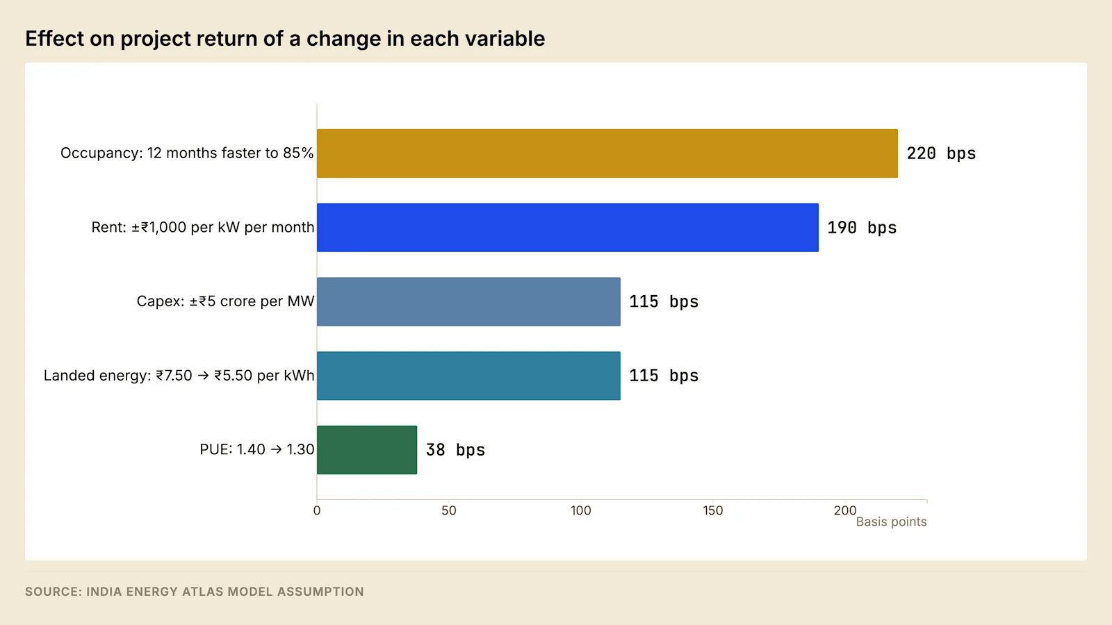
The ordering is stable across reasonable variations in the assumptions. Occupancy timing dominates because it affects the whole asset over the period when the capital is most exposed. Rent matters materially but applies only to capacity actually let. Capital cost and energy cost matter less than commonly assumed, and power usage effectiveness matters least of the five in direct financial terms, although it carries contractual significance under leases containing a PUE cap.

The energy line warrants separate examination despite its modest sensitivity ranking. Open access and group captive structures deliver landed costs materially below state utility supply, and on a block of this size the annual difference exceeds the entire non-energy operating budget. Whether that difference accrues to the operator or to the tenant is determined by the drafting of the lease rather than by any engineering decision, which makes it a legal question with a large financial consequence. Post 7 sets out how the landed cost is assembled charge by charge.

State incentives compound the same effect. Gujarat's Data Centre Policy 2026–29 provides a power tariff subsidy, reimbursement of electricity duty over twenty years, a capital subsidy, and the ability for eligible developers to hold an independent distribution licence, subject to a minimum approved IT load and a renewable sourcing condition. On the consumption profile modelled above, the tariff subsidy alone approaches two-thirds of the non-energy operating budget.

Field note. In a cost pass-through lease, a state power tariff subsidy granted against the operator's capital investment flows to the tenant by default, because the tenant is billed at landed cost and the subsidy reduces landed cost. Operators have executed twenty-year leases that transfer a state incentive, granted in consideration of the operator's investment, directly to a tenant's energy bill. The definition of "consumer" for the purposes of incentive eligibility should be settled explicitly in the lease before execution.

7.1 The method behind a one-at-a-time table #

The chart above is a one-at-a-time sensitivity. Each variable is moved from its base value while every other variable is held where it was. The instrument measures the gradient of the model at the base case, and it is the correct instrument for ranking variables by the management attention they deserve. It is the wrong instrument for measuring risk, for three reasons that operate independently of one another.

Correlation is suppressed. The variables move together in the world and separately in the table. A weaker rupee raises the capital cost of imported plant and raises the reinstatement value on which insurance is assessed. A soft leasing market lowers the achievable rent and lengthens the ramp at the same time, because the same absence of demand produces both. A one-at-a-time table presents a rent reduction and a ramp extension as two independent events with independent likelihoods, when in the state of the world that matters they are a single event with a single cause.

Interaction is suppressed. The effect of a rent reduction depends on the occupancy at which it applies, and the effect of an operating cost increase depends on how much revenue is available to absorb it. The gradient measured at the base case is not the gradient at the point where the model will actually be tested, which is a long way from the base case in the direction that hurts.

Only the axes are explored. A one-at-a-time table walks outward along each axis from the base case and never visits the interior of the space. Covenant breaches and funding shortfalls sit in the corners, where several variables have each moved moderately, rather than at the ends of the axes, where one variable has moved a long way on its own.

Model assumption — two single moves and their combination at stabilised occupancy, reference block

Neither single move removes as much as an eighth of stabilised earnings. Together they remove more than a fifth, and the coverage ratio falls far enough to engage the lock-up provisions a facility of this kind carries, whose mechanics are in Post 12. A sensitivity table reporting only the second and third rows has reported the two outcomes least likely to occur in isolation and omitted the one that determines whether the financing holds.

A further property of the instrument determines the ordering it reports, and it is worth stating because the ordering is what most readers take away. A tornado chart ranks variables by the effect of the range assumed for each, so the ranking is a joint statement about the model and about the ranges chosen. Two analysts working from an identical model with different ranges produce different orderings, and neither is wrong. The defensible form of the chart states the range beside each bar together with the basis for it, so that a reader can establish whether a variable leads the ordering because the model is sensitive to it or because the range assumed for it was wide.

7.2 Scenario construction on a correlated variable set #

A scenario is an internally consistent state of the world in which several variables take the values that state implies. Constructing one requires a causal account rather than a set of percentages, because the purpose of the exercise is to move together the variables that move together.

Three steps produce a defensible scenario. Identify the driver: a leasing market that softens, a currency that weakens, a connection that slips. Trace every variable in the model that the driver touches, including the ones it improves. And state the variables the driver does not touch, so that the scenario is bounded rather than a general pessimism.

The second step is the one most often skipped, and skipping it produces a scenario nobody acts on. A weaker rupee raises the capital cost of imported plant and raises the rupee value of any lease priced against a foreign reference. A slower leasing market lowers rent and lengthens the ramp, and it also defers the fit-out capital and the operating cost of the halls not yet commissioned. A case in which every variable moves adversely and none of the offsetting effects appears is an arithmetic exercise rather than a state of the world.

Model assumption — two single-driver scenarios and their combination, at stabilised occupancy

Two features of the table carry more information than the yield line does. The two single-driver scenarios produce the same cash-on-cash return by different routes: the first reduces the numerator while the equity stays where it was, and the second leaves the numerator almost intact while raising the equity, because construction cost above the facility commitment is funded by the sponsor rather than by the lender. And the coverage ratio behaves differently in the two cases, falling in the first and barely moving in the second, so a covenant package tested against the cost scenario alone would find nothing wrong with a project whose equity return has fallen by a quarter.

The combination is the case worth funding against. It is not the sum of the two, because the drivers touch different lines of the model, and it produces a cash return a little above half the base case while leaving the asset solvent throughout. That combination of outcomes is characteristic of this asset class: the failure mode is a return that disappoints rather than a facility that defaults, which is why equity discipline at the point of sizing matters more than covenant discipline afterwards.

7.3 Switching values and the distance to a threshold #

A switching value is the level at which a variable carries a decision from one side of a threshold to the other. It answers the question a sensitivity table does not: not how far the result moves when an input moves, but how far the input has to move before the answer changes.

The threshold used below is a coverage ratio of 1.50× at stabilised occupancy, selected to demonstrate the method. The level at which a facility locks up or defaults is set in the facility agreement, and the covenant package that sets it is in Post 12.

Model assumption — the move required in each variable, taken in isolation, to reach the stated coverage

The ordering of the switching values differs from the ordering of the sensitivities, and both orderings are correct. A sensitivity ranks by the effect of a plausible move. A switching value ranks by the distance to a threshold. Non-energy operating cost has a modest sensitivity and a very long distance to travel, so it warrants little attention in a financing discussion however carefully it is budgeted. Rent and occupancy have both a large sensitivity and a short distance, and they are where a covenant is actually lost.

The final row states a structural property of the pass-through lease rather than an arithmetic curiosity. Where energy is recovered at landed cost, the operator's exposure to the energy price is limited to the handling margin it retains, so no movement in the tariff can breach a coverage covenant. The same structure that removes the operator's exposure also removes its incentive to reduce the cost, which is the point made in section 3 and examined in Post 7.

Development cost does not appear in the table, and the reason is instructive. A cost overrun does not change EBITDA, so it does not change the coverage ratio; it changes the equity contributed and therefore the return on it, by the mechanism visible in the second scenario in section 7.2. The threshold against which development cost should be tested is a yield rather than a coverage ratio, and the natural one is the yield at which a stabilised buyer would purchase the asset, because at that point the development spread is extinguished and the sponsor has built for nothing. On the exit yield used in Post 12, development cost would have to rise by more than half before that occurred. Cost overrun in this asset class is therefore an equity return problem rather than a solvency problem, which is the opposite of the intuition most cost control effort is built on.

7.4 Probabilistic treatment and its input requirement #

A probabilistic model assigns a distribution to each uncertain input, samples them jointly, and reports the distribution of the output. Its product is a probability rather than a point: the likelihood that coverage falls below a covenant in any year, the likelihood that the equity return falls short of a hurdle, the capital at risk at a stated confidence. Where the inputs support it, this is the most informative of the four instruments in this section.

The fourth row is the limitation that matters most in this asset class. The events determining whether a project fails are discrete: the connection is energised or it is not, the anchor tenant signs or it does not, the covenant is breached or it is not. A continuous distribution over rent and occupancy prices the ordinary variation around a case in which the project works, and prices none of the cases in which it does not. The correct treatment of a discrete event is a decision tree with a stated probability on each branch, or a stress case examined on its own terms, rather than a term buried inside a sampled distribution.

Two failure modes follow from the second row. An analysis run with independent inputs understates the tails, because the adverse states of the world move several variables at once, and the joint move in section 7.1 is the elementary case of that. An analysis run with an assumed correlation matrix produces tails determined by the assumption rather than by evidence, and the assumption is almost never shown alongside the output it generated.

The practical sequence for a model of this size is ordered by what each step costs and what it returns. Rank the variables one at a time, to establish where management attention belongs. Build two or three scenarios on causal drivers, to establish what an adverse state does to coverage and to the equity return. Compute switching values against the thresholds that actually bind, which are the covenant and the equity hurdle rather than any round number. Treat the discrete events separately, as events with probabilities and responses. A probabilistic layer above those four adds precision to the output without adding information to the input, and it earns its place only where the distributions and the correlations behind it can be evidenced.

8. Boundaries of the model #

Stating what a model excludes is what makes it usable by someone other than its author.

The model is stated at the accuracy of a parametric estimate. Its capex composition is built from rates rather than from a priced design, which places it on the concept-design rung of the ladder in section 2.3. Its intended uses are screening, comparison, and the interrogation of a figure someone else has produced. It does not support a budget, a lump-sum price or a debt commitment, and a project reaching any of those stages replaces it with an estimate priced from its own drawings and accompanied by its own basis of estimate.

It excludes corporate and platform overhead. The operating cost stack in section 4 covers the facility, and an operator running several facilities carries a head office, a sales function, a treasury and a compliance function above them. Those costs are recovered from the assets and do not appear in an asset-level EBITDA, which is why an asset-level yield and a platform-level margin are not the same measurement and why the multiples applied to each differ, as set out in Post 12.

The model excludes land appreciation, which has been a material component of realised returns in Navi Mumbai and along the Chennai OMR corridor, and which is properly treated as a separate real estate position rather than as data centre income.

It excludes the tax position, which is material. Two provisions introduced in 2026 change after-tax return, and both carry eligibility conditions that determine which structures qualify. They are set out in Post 12, which is where the after-tax position and the capital structure are treated together. A yield on cost figure of the kind derived here is pre-tax by construction and should not be compared with an after-tax return from another source.

It excludes the residual value of the asset at the end of the modelled period. A data centre at the end of a twenty-year lease has a building, a power connection and a partially depreciated power train, and the value of that combination depends principally on whether the connection can serve the density the market then requires. A facility whose distribution cannot be economically upgraded is worth its land and its connection rather than its book value.

It assumes a single contract structure throughout. A facility letting part of its capacity wholesale and part retail carries a blended energy treatment, and the margin optic described in section 3.2 becomes a weighted average that no single figure represents.

It assumes that power is delivered on schedule, which frequently does not occur. CEEW's 2026 assessment records that developers continue to report delays in land acquisition, building approvals, grid connectivity and fire safety clearance notwithstanding single-window provisions. A delay to energisation does not simply postpone revenue: it postpones the start of the ramp, so the loss compounds across the following years rather than being recovered in them. At sector level, the India Data Centre Review 2026 estimates the pipeline effect of a six-month connection delay in hundreds of MW. Post 3 sets out the connection process and where it fails.

Field note. The electrical and mechanical packages together constitute the majority of project cost, and the facility exists to deliver conditioned, uninterrupted power to computing equipment. Cost reduction exercises that concentrate on the building fabric address a minority of the capital and leave the majority untouched. Where the power train is simplified to reduce cost, the resilience class changes, and with it the population of tenants that will lease the facility and the yield at which an institutional buyer will underwrite it.

Forward look #

Three developments over the next eighteen months would alter the assumptions in this model, and each is observable in advance.

The first is whether absorption in 2026 clears the level Savills projects, which would indicate that the ramp assumptions used here are conservative and that the sensitivity ordering in section 7 understates the value of anchor tenancy.

The second is whether the revived National Data Centre Policy at MeitY converts from consultation to notification, and in particular whether the proposed Data Centre Economic Zones with pre-provisioned power and single-window clearance are implemented. If they are, the energisation delay risk discussed in section 8 becomes materially smaller for facilities inside those zones and materially larger for facilities outside them.

The third is whether leasing at high rack densities begins to reprice the rent line upward, or whether it raises capital cost per MW without a corresponding increase in rent. The second outcome would compress yields across the sector, because it increases the denominator of the yield calculation without affecting the numerator.

FAQ #

What does a data centre cost per MW in India? Between ₹55 crore and ₹70 crore per MW of IT load for hyperscale-grade colocation at current pricing. Electrical and mechanical systems account for the majority of that figure. The resilience layer required to bridge grid availability to contracted availability accounts for a further tenth to sixth of project cost.

How much revenue does one MW of Indian data centre capacity generate? Contracted rent is billed per kW of reserved capacity per month and is charged whether or not the capacity is drawn. Energy is recovered separately in most wholesale contracts. Revenue per MW therefore depends on the contract structure as much as on the rate achieved.

What is a normal yield on cost for an Indian data centre? Mid-teens at stabilised occupancy on the model set out above. Project internal rate of return depends considerably more on how quickly the asset reaches stabilised occupancy than on the stabilised yield itself.

Why do published estimates of India's data centre capacity disagree? They measure different quantities. Colocation IT load, total facility power and sanctioned grid load differ systematically, and the ratios between them are set out in section 1. Any comparison requires the denominator to be established first.

Does the tenant or the operator benefit from a state power tariff subsidy? It depends on the lease. Under a cost pass-through structure the benefit reduces the tenant's bill by default. The definition of "consumer" for incentive purposes should be negotiated explicitly.

What is included in a data centre cost per MW figure? It depends on the boundary applied. An EPC contract value, a total installed cost and a total development cost describe the same building and differ by owner's costs, land and finance. The range quoted in this post sits on the widest of the three. Section 2.5 sets out the bridge between them and the lines most often omitted.

Sources #

• Savills India, India Data Centre Market Update H1 2026, July 2026

• Houlihan Lokey, Data Center India Edition, December 2025

• Mordor Intelligence, India Data Center Market Report, June 2026

• Eninrac, India Data Center Market 2026–2030, June 2026

• IMARC Engineering, Data Center Development in India, June 2026

• Government of Gujarat, Data Centre Policy 2026–29, June 2026 (via NASSCOM Public Policy)

• CEEW, India Data Centre Analysis 2026

• Finance Act 2026 and Union Budget 2026 provisions on notified data centres

• India Data Centre Review 2026 (v2.3, edition cutoff 28 July 2026), Chapters 1, 4 and 5 — India Energy Atlas

• Global Data Center Hub, Q1 2026 capital tracker, via IDCR 2026

• JLL, India Data Centres H1 2025 dynamics, via IDCR 2026

• AACE International, recommended practice on cost estimate classification — named at instrument level in section 2.3; no accuracy band from it is reproduced

• FIDIC, conditions of contract — named at instrument level in section 2.4 as one of the standard form families

Capex composition, the operating cost stack, the revenue build-up, the occupancy ramp, the estimate-class ladder, the escalation and phasing arithmetic, the lease pricing calculation, the churn and receivable arithmetic, the coverage profile and the sensitivity, scenario and switching-value analysis are modelled by India Energy Atlas and are labelled as model assumptions throughout. They are not attributed to any external source. IDCR 2026 figures are quoted at the locked edition snapshot of 13 July 2026; live Atlas products may carry newer records.

Read the full series — The Indian Data Centre Playbook, twelve parts from unit economics to exit.

Next in the series — Part 2: Site Selection Is a Power Problem. Screening substation headroom, transmission corridor capacity and water availability before land is committed.

India Energy Atlas builds India's grid intelligence layer — substation headroom, interconnection queues, market prices, and carbon intensity in one place. See energymap.in/pricing.