Power Procurement for Indian Data Centres: The Landed Cost Stack from PPA to Meter

The short answer. The generation tariff in a power purchase agreement is a minority of what a data centre pays at the meter. Cross-subsidy surcharge, additional surcharge, wheeling, transmission, losses and banking terms complete the delivered cost, and they vary by state to the point where an identical structure is economic in one jurisdiction and uneconomic in another. Procurement structure should be selected against landed cost rather than against generation tariff.

This post sets out how the delivered cost of electricity is assembled for a large Indian consumer, which components are negotiable and which are not, and how the available procurement structures compare on the basis that matters. It is written for the energy manager structuring supply, the developer modelling operating cost, and the investor testing whether a stated ₹/kWh assumption is credible.

The central point is that the headline tariff in a power purchase agreement is a component of the delivered cost rather than a proxy for it. Comparisons conducted on generation tariff rank states and structures in an order that the landed cost does not support, and the error is systematic rather than random because the largest charges fall on the structures with the lowest generation tariffs.

1. The charge stack #

Electricity procured under open access is delivered over a network the consumer does not own, from a generator the consumer does not own, and each party in that chain levies a charge.

Two components dominate the difference between states. Cross-subsidy surcharge compensates the distribution licensee for the cross-subsidy it no longer collects from a consumer who has left its supply, and additional surcharge compensates it for fixed costs incurred to serve a consumer who is no longer taking supply. Both are set by the state electricity regulatory commission, both are revised periodically, and both are large enough in some states to eliminate the entire advantage of open access procurement.

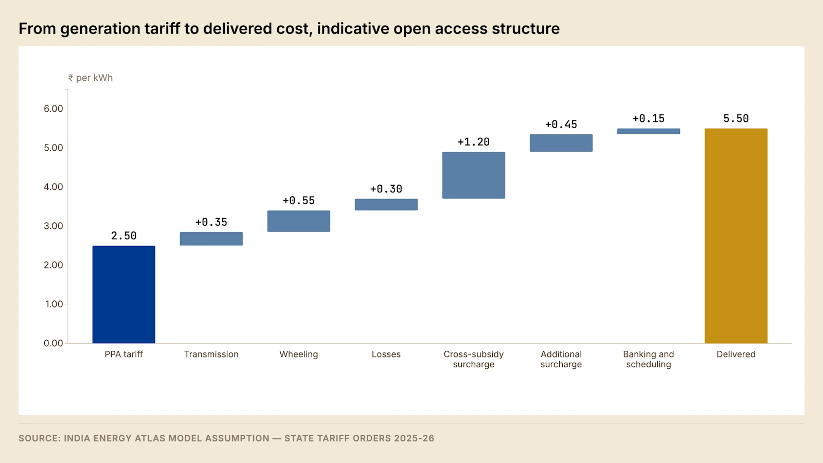
The stack is what converts a competitive generation tariff into a delivered cost that may or may not beat the distribution licensee's industrial tariff. A procurement decision taken on the first line of the stack, without the remaining lines applied, is not a procurement decision.

1.1 Statutory basis of each component #

Each line of the stack is levied under its own instrument, by its own authority, on its own revision cycle, so no single order states the delivered cost.

Record the instrument and its effective period against every line of the model, because a figure carried without one cannot be refreshed or defended.

1.2 Computation of the cross-subsidy surcharge #

Cross-subsidy surcharge is computed on a formula prescribed in national tariff policy and adopted, with state variation, by each commission. It is the difference between what the departing consumer paid the licensee and what it cost the licensee to serve that consumer at the margin, with marginal power purchase cost grossed up for losses to the consumer's voltage and the separately recovered charges deducted.

Three properties follow. The surcharge is largest for the categories that cross-subsidise most, because the first term is the consumer's own category tariff, and a data centre takes supply in a high-tension category whose tariff sits above the cost to serve. Decarbonisation of the licensee's portfolio does not reduce it, because renewable generation is excluded from the marginal cost term. Both the tariff term and the loss term are voltage-specific, so a change of connection voltage moves two terms at once.

The failure mode is a model built on the surcharge in force at term sheet, since the determination is revised with the tariff order and no consumer holds a vested entitlement to it. The Green Energy Open Access Rules, 2022 limit how far the surcharge may be raised above the level prevailing when access was granted.

The diligence question is which order determines the surcharge for this consumer's category and voltage, and when the next determination falls due. A rupee value carrying no instrument belongs in the model as an assumption rather than as a fact.

1.3 Determination of the additional surcharge #

Additional surcharge is levied under Section 42(4) of the Electricity Act, 2003 on the charges of wheeling, and it compensates the distribution licensee for fixed costs it continues to carry under its obligation to supply after the consumer has left.

The mechanism is contracted capacity. A licensee procures generation in advance against a projected demand and pays the capacity charge whether or not energy is taken, so the fixed cost attributable to a departed load is stranded until the capacity is sold, surrendered or absorbed by demand growth.

Three features of the determination govern the exposure. The licensee must demonstrate on evidence that the cost has actually been stranded, which is harder where its demand is growing than where it is flat. The determination follows a petition rather than the annual tariff exercise, so it arrives on its own cycle. The commission fixes the date from which the charge applies, and that date can precede the order.

The petition is contested, and the commission tests it on an evidentiary record rather than on the licensee's assertion. Four propositions have to hold together before a charge is determined, and an objector attacks each of them separately.

The third and fourth propositions carry most of the argument. A licensee holding surplus contracted capacity may sell it, and the revenue earned reduces the stranded cost the surcharge is meant to recover, so the treatment of those sales moves the determination directly. A licensee whose approved revenue requirement already recovers the same capacity charge from its remaining consumers cannot recover it a second time from those who have left, and the reconciliation between the two filings is where a well-argued objection concentrates.

The quantum is expressed as a rate on the open access consumer's drawal, so the charge scales with energy taken rather than with capacity contracted. A load with a high load factor therefore carries more additional surcharge for each MW of contract demand than an intermittent load of the same size, which is the reverse of the pattern in which the stranded cost was incurred, and it is the reason this charge falls heavily on a continuously operating facility.

The commission also fixes the period the determination covers and the date from which it applies, and both are contested. A determination applying from a date preceding the order creates a liability for consumption already taken and already billed, which the consumer can recover from nobody. Where a petition has been filed and is pending, the exposure is live even though no charge is being levied, and the pendency is itself the evidence a model should carry.

Where no determination is in force the correct treatment is a stated downside case rather than a zero, and the best evidence of future exposure is the licensee's contracted capacity position against its own demand forecast, both on the record in its tariff petition. The failure mode is a model built with no additional surcharge because none was in force when it was built; it surfaces when a determination issues with effect from an earlier date, by which time the consumption is historic and the exposure is arithmetic.

1.4 Wheeling, losses and the voltage of delivery #

Wheeling charge is levied by the distribution licensee for use of its network and is payable only on the part of the delivery that uses that network. It is determined by voltage level, because a consumer connected at a higher voltage uses fewer network elements.

Connection voltage is therefore a procurement variable and not only an engineering one. A consumer drawing at extra-high voltage from the transmission system does not use the distribution network for its bulk supply and attracts no wheeling charge on it. Connection voltage follows from the firm capacity requirement derived in Post 2, through the process described in Post 3.

The failure mode is a model that applies one loss percentage to a delivery crossing two or three networks. Losses apply successively rather than additively, so the gap widens with every boundary crossed. The diligence request is the energy accounting statement of an existing consumer under the same structure in the same state.

1.5 Standby charges and retained contract demand #

An open access consumer does not cease to be a consumer of the distribution licensee. It retains a connection for the periods in which its contracted supply is unavailable and pays for that availability in two ways: a demand charge on the contract demand retained, payable whether or not energy is drawn, and a standby rate on energy drawn outside the open access schedule, set at a premium to the retail rate in several states.

For a data centre the retained demand is not discretionary, because the facility cannot be unserved when its contracted generation fails. The demand-charge component of the licensee's bill therefore largely survives the move to open access, and only the energy-charge component is displaced.

This is the most common overstatement in a quoted open access saving. The saving is computed against the full retail tariff with demand charges included, while those charges continue to be paid on the retained connection. The correct comparison carries the retained demand charge on both sides, so the saving reduces to the difference in the energy-charge component.

The diligence questions are what contract demand is retained, at what demand charge, whether a standby rate applies to energy drawn outside schedule, and on what notice contract demand may be reduced. Contract demand is routinely registered against rated design capacity rather than measured peak, for the reasons set out in Post 2.

1.6 Build-up from generation tariff to meter #

Model assumption — delivered cost of an intra-state renewable open access structure, moderate-surcharge state, ₹ per kWh

Source: India Energy Atlas model assumption, calibrated on state tariff orders for 2025-26 and on India Data Centre Review 2026, Chapter 5.

The generation tariff is under half of the delivered cost, and the two surcharges together exceed transmission, wheeling and losses combined. The result sits close to the national weighted average industrial tariff of ₹5.6 per kWh in the CEA tariff order for FY2025, so in a moderate-surcharge state the structure is near parity and the case for it rests on term certainty rather than on an immediate saving. The build-up excludes electricity duty, the retained demand charge from section 1.5 and deviation settlement.

1.7 The multi-year tariff framework and the control period #

Wheeling and transmission charges are not fixed year by year in isolation. A state commission determines them across a control period spanning several years, approving at the outset a trajectory for the parameters within the licensee's control and providing for the parameters outside that control to be passed through as they arise.

The division between the two categories decides who bears a variance. A licensee that betters an approved efficiency trajectory retains a share of the gain and one that misses it absorbs a share of the loss, so the approved trajectory rather than the outturn drives the charge for most of the period.

Three consequences follow for a procurement model. A wheeling charge has an approved forward path already on the record, so a model can be built on the trajectory and refreshed against each annual order rather than assuming the current year continues. The boundary between one control period and the next is the point of largest movement, because the base is re-determined rather than extended. And a power purchase agreement running for two decades spans several control periods, so the charge stack in the model is a forecast across most of the contract term whatever the first year shows.

The surcharges do not follow this cycle. Cross-subsidy surcharge moves with the retail tariff order because its formula draws on that order's own terms, and additional surcharge moves on a petition with a timetable of its own. A model that refreshes the network charges on the control period and leaves the surcharges static has refreshed the smaller half of the stack.

The diligence questions are which control period is running, when it closes, and what trajectory was approved for the loss level and the wheeling charge. The retail tariff determination that supplies the surcharge inputs is set out in Post 2.

1.8 The annual revenue requirement and the true-up cycle #

The licensee's revenue requirement is approved before the year begins, incurred during it, and reconciled after it closes. The reconciliation is the true-up, and it is the mechanism by which a cost arising in one year reaches a charge levied in another.

Three properties of the cycle bear on an open access consumer. The lag between the year a cost arises and the year it is recovered commonly exceeds a single year, so a charge in force today can be carrying recovery for a period during which the consumer was taking supply under a different structure. The carrying cost on a deferred gap accrues, so a licensee with a large regulatory asset holds a claim that grows rather than a static one. And the categories from which a gap is recovered are selected in the recovery order, which tends to place the burden on the categories able to bear it.

The link to the surcharge is direct rather than indirect. Every term of the cross-subsidy surcharge formula set out in section 1.2 is an output of this cycle: the category tariff, the marginal power purchase cost, the loss level at the delivery voltage, the wheeling charge and the regulatory asset carrying cost. A true-up that revises power purchase cost revises a surcharge input, so a consumer that has left the licensee's supply remains exposed to that licensee's cost recovery for as long as the formula stands.

The failure mode is a model refreshed from the current tariff order alone. That order states the charges in force; it does not state the pending true-up petitions, the approved regulatory asset balance or the recovery schedule, and those three determine the direction of the next revision rather than its existence. The diligence set is the tariff orders for the last three years, the true-up orders sitting alongside them, and the regulatory asset balance the commission has approved.

1.9 Energy accounting between the four parties #

A unit delivered under open access is metered at more than one point and accounted for by more than one party, and the delivered cost in section 1.6 is assembled from documents each of them issues separately.

The account is assembled in a fixed order, and the order changes the answer. Injection is established first at the generator's meter. Losses are applied to bring the injected quantity to the point of accounting, which reduces the units available to the consumer without appearing anywhere as a charge. Drawal is established at the consumer's meter. The two quantities are then compared block by block, matched drawal is treated as supplied under the contract, and the residual in either direction goes to banking, to the licensee at the standby rate, or to deviation.

Losses applied in kind and losses charged in cash produce different invoices for identical physics. Applied in kind, a loss reduces the units the consumer receives, so the consumer contracts for more energy than it consumes and pays the generation tariff on the difference. Charged in cash, the units arrive intact and a separate charge appears. The delivered cost reconciles between the two treatments only where the loss percentage and the generation tariff are both stated on the correct basis, and a model that applies a cash loss charge in a state operating in kind counts the loss twice.

Three reconciliation defects recur. Meter time drift places energy in the wrong block, which matters because matching, banking and deviation are all block-level operations rather than monthly ones. A meter installed away from the point at which charges are computed produces an account that cannot be tied to the invoice, which is one of the refusal grounds in section 8.1. Missing meter data is filled by an estimation procedure whose output binds unless it is challenged inside the objection window.

The diligence question is not whether the consumer receives an energy account but whether anybody reconciles the four documents against each other. The generator's invoice, the licensee's bill, the state energy account and the facility's own metering all describe the same month, and a difference between them is either a defect nobody has found or a charge nobody has identified.

2. The same structure across states #

Applying an identical solar open access structure across Indian states produces delivered costs that differ substantially, and in at least one major market the structure is more expensive than simply taking supply from the distribution licensee.

Source: state tariff orders for 2025-26, via IDCR 2026, Chapter 5.

The same six states expressed as a delivered cost rather than as a set of levels give the ranking directly.

Source: IDCR 2026, Chapter 5, from state tariff orders.

The two right-hand columns rank the states differently, because the second compares against a licensee tariff that itself varies. A state can carry a high landed cost and still show a saving where the licensee's own tariff is higher still. The two columns answer different questions: the first governs what the facility will pay once built, the second governs whether arranging open access in that state is worth the effort at all, and a developer that has already committed to a location needs the first while a developer still choosing between locations needs both.

Maharashtra is the case worth studying, because it carries among the most competitive solar generation tariffs in the country and the least attractive delivered cost. A high cross-subsidy surcharge combined with monthly banking destroys more value than the generation advantage creates. A developer ranking states on power purchase agreement tariff would place Maharashtra near the top. A developer ranking on landed cost places it last, and behind the distribution licensee's own tariff.

Banking terms deserve more weight than they usually receive in structuring discussions. Solar generation is concentrated in the middle of the day and a data centre load is essentially flat, so the two profiles do not coincide. Banking is the mechanism that reconciles them: energy generated in excess of consumption is credited and drawn down later. A twelve-month banking period allows seasonal reconciliation. Monthly banking allows almost none, and a "none" provision forces the structure into a hybrid or storage-firmed design from the outset. The nominal saving from a low generation tariff can be entirely consumed by the cost of managing an unbankable surplus.

2.1 Banking settlement mechanics #

Banking is an accounting arrangement with a settlement procedure, a series of deductions and an expiry, rather than storage.

Energy accounting is performed against metered injection and drawal in each time block. Drawal matched by injection within the block is treated as consumed directly. Injection in excess of drawal is credited to the bank, and drawal in excess of injection is met from the bank where the state permits withdrawal in that period and otherwise from the licensee at the standby rate.

Four consequences follow for a flat load. A banked unit is worth less than a directly consumed unit by the sum of every row above rather than by the banking charge alone. The time-of-day restriction binds hardest, because a continuous load consumes through the evening peak, which is the period in which withdrawal is most often prohibited. Only a settlement period spanning the monsoon allows a pre-monsoon surplus to meet a monsoon shortfall. The lapse rate is commonly the licensee's average power purchase cost, so unrecovered energy is settled below the contracted tariff.

The sizing rule is to design generation against recoverable banking rather than against nominal entitlement. The diligence questions are the settlement period, any restriction by time of day or season, the banking charge, the treatment and price of unutilised credit, and whether the provision continues for the term of the power purchase agreement. Banking is a policy provision rather than a contractual one, and revisions have bound existing consumers.

2.2 Worked landed cost in a low-surcharge state #

The build-up in section 1.6 uses a state with moderate surcharges. Repeating it against each end of the published range separates the part of the difference between states that arises in the stack from the part that arises in the generation tariff, because the generation tariff is held identical across both instances.

Model assumption — delivered cost in a low-surcharge state, ₹ per kWh

Source: India Energy Atlas model assumption. Every component sits inside the ranges reported in section 1.6, and the total corresponds to the published landed cost for Karnataka in the table above.

The assumption set is the model's rather than the published source's, and it is stated line by line so that a reader can substitute a particular state's own orders without rebuilding the structure of the calculation.

Two properties of the low-surcharge case deserve attention. The two surcharges together are smaller than the network charges, which reverses their relative position in the moderate case, and about three-quarters of the gap between the two states arises in the surcharge lines rather than in the network lines. A twelve-month banking period is also doing work that appears in no line of the table, because it converts a midday surplus into an evening unit at the banking charge rather than at whatever the exchange happens to clear.

A published instance for the same state offers an independent check on the order of magnitude.

Source: IDCR 2026, Chapter 5.

The instance states a load and two prices without the utilisation and the hours behind its energy quantity, so it cannot be reproduced arithmetically from what is published. A reader rebuilding a saving of this kind should state the utilisation, the design efficiency and the hours explicitly, which is what section 2.4 does.

2.3 Worked landed cost in a high-surcharge state #

Model assumption — delivered cost in a high-surcharge state, ₹ per kWh

Source: India Energy Atlas model assumption. The total corresponds to the published landed cost for Maharashtra, the state in the table above whose delivered cost exceeds the licensee's own tariff.

The generation tariff is identical to the low-surcharge instance by construction, so the whole of the difference of ₹2.30 per unit between the two instances arises in the stack. Cross-subsidy surcharge alone exceeds the entire network charge in this instance, and it is the single line on which the structure turns.

Monthly banking compounds the position. A surplus that cannot be carried past the month is either sold at the prevailing exchange price or lost, and the months in which a solar structure runs its largest surplus are not the months in which the exchange clears highest. The generation advantage is reduced once by the surcharge and again by the terms on which surplus energy has to be disposed of, and neither reduction is visible in the tariff that attracted the developer to the state.

The failure mode here is a structure signed before the surcharge determination applicable to the consumer's own category and voltage has been read. The generation tariff is contracted for the term and the surcharge is not, so the delivered cost in the model is a forecast whose largest single line is also its least certain.

2.4 Annual cost of the two instances on the reference block #

Converting the two instances into an annual amount requires the facility's consumption, which follows from the reference block used throughout this series.

Model assumption — annual energy cost of the reference block under each instance

The block size, the utilisation and the design efficiency are the series constants set in Post 1. The delivered costs are the two instances above.

The difference between the two states on an identical contract exceeds the entire non-energy operating cost of the reference block, which Post 1 derives. That places the choice of state alongside the choice of structure rather than beneath it, and it is the arithmetic underneath the site-selection screen in Post 2. The recurring difference capitalises at the exit yield, which Post 12 sets out.

Two boundaries apply to the comparison. Both instances assume the structure supplies the whole of the facility's consumption, which no renewable open access structure achieves without storage or a hybrid portfolio, so the realised difference scales with the share actually supplied. And both exclude electricity duty, the retained demand charge from section 1.5 and deviation settlement, for the same reason section 1.6 excludes them.

3. The ISTS waiver phase-out #

The waiver of inter-state transmission system charges for renewable generation has been the largest single subsidy supporting inter-state renewable procurement, and it is being withdrawn on a published schedule.

The mechanism matters for project modelling. The waiver applicable to a project is determined by its commissioning date, and the schedule steps down at fixed intervals. A project modelled at the waiver applicable when the term sheet was signed, but commissioned after a step-down, carries a transmission charge the model does not contain. Given the connection timelines set out in Post 3, the gap between those two dates is routinely long enough to cross a step.

The correct modelling practice is to apply the waiver applicable to the commissioning date the project will actually achieve rather than the date in the plan, and to carry the difference as a downside case. The waiver withdrawal also changes the relative economics of inter-state and intra-state procurement, because intra-state structures are unaffected by it. Where a state has adequate renewable resource, the withdrawal narrows and eventually removes the case for sourcing across a state boundary.

3.1 The step-down schedule and the commissioning-date test #

Source: Mercom India, March 2026.

The schedule operates as a series of cliffs rather than as a continuous decline. The waiver is fixed by the commissioning date and runs from it for a stated period, so a project missing a window by a short interval carries the next step for its whole operating life. Withdrawal adds approximately ₹0.40 to ₹0.50 per unit to an inter-state renewable supply on the assessment published by pv magazine India in September 2025.

A station whose storage is charged from the renewable plant at the same substation carries a full waiver over twelve years, subject to a limit on the share of charging drawn from the grid, which preserves the advantage of a firmed inter-state supply after the waiver on unfirmed supply has stepped down.

The failure mode lies in allocation rather than in size. Where the generator has priced the waiver into its tariff and the project commissions after a step, the change-in-law clauses of the two agreements decide which party bears the charge.

3.2 Storage co-located with generation and the treatment of its charges #

Section 3.1 states the waiver position for storage charged at the same substation as the renewable plant. The conditions attaching to that waiver are operating conditions rather than design conditions, so compliance has to be enforced in the despatch logic and evidenced in the energy account rather than inferred from the physical arrangement.

Source: Mercom India, March 2026.

Storage changes both the profile delivered and the charges that attach to it, and the two effects settle under different instruments. Reading the stack in section 1 against a stored unit rather than a directly injected one shows which lines apply once and which apply twice.

The metering point decides how the arrangement is accounted for. Storage behind the generator's interface meter is invisible to the network, and its effect appears only as a change in the shape of the injection, so the charge stack applies once and applies to the delivered profile. Storage on the consumer's side of the point of supply is a different structure altogether: it charges from units that have already borne the whole stack, and any energy exported from it re-enters the network as a fresh injection with its own accounting consequences.

The round-trip loss is the cost most often omitted. A unit stored and later recovered reaches the meter reduced by the storage efficiency as well as by the network losses, so the delivered cost of a firmed unit exceeds that of a directly injected unit by more than the storage tariff alone. The contract has to state whether the generation tariff is payable on units injected into storage or on units delivered from it, because the difference between those two bases is the round-trip loss and it accrues for the term.

Storage and banking are substitutes, and the value of the first is set by the terms of the second. Where a twelve-month banking period is available at a modest charge, storage competes against a cheap alternative and the case for it is weak. Where banking is monthly or unavailable, storage becomes the only mechanism that carries a midday surplus into an evening hour, and its value is the difference between the contracted tariff and whatever that surplus would otherwise realise. The state comparison in section 2 therefore drives the storage decision as much as the cost of the storage does.

Cell chemistry, containment and the interaction with backup duty are set out in Post 6, and the value of the same asset in system services is set out in Post 10. The point here is narrower: an identical physical asset attracts a different set of charges according to which side of a meter it sits, so the siting decision is commercial before it is technical.

The diligence questions are where the storage is metered, who owns it, whether the tariff is struck on units in or units out, which party bears the round-trip loss, what evidences compliance with the grid-charging limit, and what becomes of the waiver if that limit is exceeded.

4. Group captive #

Group captive operates under Section 9 of the Electricity Act, 2003 and the Electricity Rules, 2005, and it exists because a consumer who owns its generation is not a consumer of the distribution licensee in the sense the surcharges contemplate.

Two conditions must be satisfied and both are tested. The captive users must collectively hold not less than twenty-six percent of the ownership of the generating plant, and they must collectively consume not less than fifty-one percent of the electricity generated, on an annual basis, in proportion to their shareholding.

The proportionality requirement is the one that fails in practice. It is not sufficient for the group as a whole to meet both tests; each captive user's consumption must correspond to its shareholding within a tolerance. A consumer whose load falls materially below forecast, for instance because an occupancy ramp has been slower than modelled, can breach proportionality without any change in the structure itself. The consequence of breach is retrospective loss of captive status and a demand for the surcharges that were not paid, which is a materially worse outcome than never having adopted the structure.

The benefit is the exemption from cross-subsidy surcharge and additional surcharge in most states, which on the stack in section 1 is frequently worth more than the entire difference in generation tariff between structures. That is why group captive is the dominant structure for large Indian consumers in high-surcharge states despite its administrative burden.

4.1 Evidencing the two conditions #

The ownership condition is tested on the shareholding of the company that owns the plant, which must be held in equity carrying voting rights and must subsist through the year rather than at a single date. The consumption condition is tested on the energy accounts, against the collective threshold and against each user's proportionality to its shareholding.

Both tests are annual, so a breach early in a year surfaces only after the year has closed and the demand covers the whole period at the surcharge rates then in force. The monitoring implication is a monthly reconciliation of each user's consumption against its shareholding, while correction remains available.

4.2 The value of the exemption #

Model assumption — landed cost by structure in a high cross-subsidy-surcharge state, ₹ per kWh

The gap between the first row and the third combines the exemption from both surcharges with the difference between a licensee's average cost of supply and a contracted renewable tariff. The gap between the second row and the third is the narrower quantity a structuring decision actually turns on, because both of those rows already carry a contracted generation tariff and differ principally in the surcharges they attract.

Expressing the exemption for each MW of IT load makes it portable to any block size.

Model assumption — value of the exemption for each MW of IT load

The last row matters because no renewable structure supplies a continuous load in full without storage or a firming contract, so the realised value scales with the share actually supplied rather than with the capacity contracted. On the reference block the resulting annual amount is the recurring saving that Post 12 capitalises at the exit yield.

The exemption has to be set against what the structure costs to run. The compliance burden is a recurring administrative cost together with a capital commitment in the generating company, and neither is a published figure for this asset class, so the correct treatment is a break-even rather than an assumed number.

The break-even consumption decides whether a load is large enough for the structure to be worth adopting. A small load carries substantially the same certification and governance cost as a large one, so the fixed element of the burden falls for each unit as consumption rises, which is the mechanism behind the observation in section 8 that group captive suits large loads in high-surcharge states.

The diligence concerns the parties the consumer does not control: the identity and load stability of the other captive users, whether the shareholding is held in voting equity, and what becomes of the structure if a user exits. A satisfactory answer produces the previous year's energy accounts and the certification filed against them. Renewable purchase obligation binds captive users directly, and is examined in Post 8.

4.3 Verification of captive status and the annual certificate #

Captive status is asserted by the consumer and verified afterwards against records rather than granted in advance, so the structure has to be operated in a way that produces the records verification depends on.

The ownership condition is verified from the generating company's register of members and its constitutional documents, which together establish the class of shares held, whether those shares carry voting rights, and the period through which the holding subsisted. The consumption condition is verified from energy accounts: the plant's generation for the year, each captive user's consumption at its own meter, and the proportionality of the second to each user's shareholding.

Certification draws the two together. A chartered accountant certifies the ownership and consumption position for the year against the audited financial statements and the metered energy records, and the certificate is filed with the state authority and with the agency that maintains the energy accounts. That certificate is the document a purchaser, a lender and an assessing authority will each ask to see.

Two properties of the verification determine when a problem becomes visible. It is annual, so a divergence arising early in the year is certified only after the year has closed. And it is documentary, so a structure that is economically sound but poorly recorded fails on the same evidence as one that is unsound.

The failure mode is a certificate prepared from the generator's own generation record and the users' internal consumption estimates without reconciliation to the state energy accounts. It presents as a certificate that cannot be tied to the accounts the licensee bills against, and it surfaces when a demand is raised and the certificate is offered in answer to it.

The diligence request is the certificate for the last completed year together with the state energy accounts for the same period, reconciled line by line. A certificate that cannot be reconciled to those accounts establishes nothing about the structure.

4.4 Change in shareholding and its effect on captive status #

The ownership condition is continuous rather than a snapshot, so any event moving the shareholding of the generating company moves the test itself.

The proportionality link is the part most often missed. Each user's consumption is tested against its shareholding, so a change in shareholding part-way through a year changes the quantity that user needed to have consumed across the whole of the year, including the months already elapsed. A transfer agreed in the final quarter can therefore create a breach for a period during which every party complied with the position as it then stood.

Two structural protections address that. Transfers can be restricted to the opening of a compliance year, so the tested position holds for the whole of it. And the shareholders' agreement can carry a restoration obligation requiring the parties to take whatever steps return the collective holding to the threshold within a stated period after any event that reduces it.

The consequence of a breach is the one stated at the head of this section: retrospective loss of status for the year, with a demand for the surcharges that were not paid. That exposure sits with the consumer even where the event causing it occurred at a counterparty, which is why the documents governing the structure matter as much as its economics.

A change of control at the data centre operator itself raises the same question from the other direction, because the consuming entity is a party to the structure and its sale becomes a condition to completion in a transaction. Post 12 sets out how change-of-control consents are handled at exit.

The diligence set is the shareholders' agreement, the transfer restrictions within it, the register of members for the last completed year, and the mechanism by which the collective holding is restored after a dilution.

Field note. A data centre in its occupancy ramp is a poor fit for a proportionality test calibrated on stabilised consumption. Where group captive is adopted before stabilisation, the shareholding should be structured against the ramp rather than against the eventual load, with a mechanism to adjust as consumption grows. Structures that assume stabilised consumption from year one breach in year one.

5. Exchange procurement #

The power exchanges provide a third channel that behaves differently from both bilateral contracting and distribution licensee supply.

Exchange procurement carries no long-term commitment and no counterparty credit exposure, and it prices at whatever the market clears. For a data centre this is attractive as a marginal channel and unattractive as a primary one, because the load is flat and continuous while exchange prices are volatile and seasonal. A facility procuring its full requirement from the exchange has converted a predictable operating cost into an unhedged commodity exposure, which is not a position an infrastructure lender will accept.

The useful application is at the margin. Exchange purchases fill the gap between contracted renewable generation and actual consumption, particularly during periods when banked energy has been exhausted. Exchange sales dispose of surplus generation where banking terms do not permit it to be carried. In both cases the exchange is managing the mismatch between a variable generation profile and a flat load, which is the same problem banking terms address by a different mechanism.

The green market segments allow renewable attributes to be procured separately from energy, which is relevant to the carbon position examined in Post 8 but which does not by itself change the delivered cost of energy.

5.1 The segments and their delivery horizons #

The exchanges are not a single market. Each segment closes at a different point relative to delivery, and the segment a consumer can reach determines how late a position can be corrected.

Source: Indian Energy Exchange market updates, 2026.

Exchange prices rise with the summer demand peak, so the annual average understates what a consumer pays in the months when it is most likely to be short of its own generation. That correlation is the reason exchange procurement cannot carry a large share of a continuous load.

CERC directed market coupling in July 2025 for a day-ahead start in January 2026, the Indian Energy Exchange appealed to the Appellate Tribunal for Electricity, and a corrigendum in January 2026 reclassified the order as directions. Coupling had not gone live at the edition cutoff, so a position taken on one exchange carries basis risk against another.

5.2 Traded volume, price level and the seasonal shape #

Three readings of the table above bear on a procurement position, and each of them changes what the exchange can safely be used for.

Volume. The exchange carries a growing but still minority share of the energy changing hands in India, because most energy moves under long-term contracts between generators and distribution licensees. A consumer relying on the exchange for a large block is taking a position against a residual pool, and a requirement large enough to move the clearing price will not transact at the published average.

Level. The annual average is the least useful figure in the table for a continuous load, because the load buys in every block of the year while the average is weighted toward blocks in which system demand is low. The figure that governs the exposure is the price prevailing in the periods when the consumer is short of its own generation.

Shape. The day-ahead and real-time segments hold no stable relationship to each other. Real time cleared above day ahead in the quarter shown in the table and below it in both summer months, so a buyer deferring cover from one segment to the other as a standing policy has taken a position on the spread rather than captured a discount. Post 10 reads the same relationship from the despatch side, where the question is which segment a load shift can be committed in.

The green day-ahead segment cleared below the conventional segment on the annual average, so the renewable attribute carried no premium at that resolution. That does not make the segment a substitute for a contracted renewable supply, because a purchase in it establishes nothing about the hour in which the generation occurred, and the hourly question belongs to Post 8.

The exchange also operates a market in attributes rather than in energy. Its volumes, clearing range and the mechanics of issuance and redemption are set out in Post 8. For procurement the only consequence is that a certificate purchase discharges an obligation without delivering a unit, so it never enters the landed cost of energy computed in section 1.6.

Two distinct periods drive the exposure and they arise from different causes. The summer months raise the price because system demand peaks. The monsoon months raise the consumer's shortfall because solar output falls. A structure exposed to both carries its highest prices and its largest volume requirement in different parts of the year, so the annual exposure has to be modelled month by month rather than at the annual average.

The practical rule is to size the exchange's role against the consequence of its worst month rather than against its average. A share of load affordable at the annual average may be unaffordable in a month clearing at the summer level, and an infrastructure lender sizing a debt service coverage test will apply the second of those.

6. Deviation settlement #

The charge stack in section 1 lists deviation settlement as an exposure rather than a fixed charge, and it is the component most often omitted from procurement models.

A consumer procuring through open access schedules its expected drawal in advance. Departure from that schedule is settled at a rate that varies with system frequency and with the direction and magnitude of the deviation, under the applicable deviation settlement mechanism regulations. The exposure is therefore a function of forecast accuracy rather than of consumption.

Measured accelerated-computing workload traces indicate that data centre load carries substantially more short-term variability than the flat profile assumed in most procurement models, because training workloads alternate computation with collective communication and inference load follows demand. A scheduling process calibrated on an assumed flat profile will deviate, and the resulting settlement is a recurring cost that appears nowhere in the term sheet.

Two mitigations are available. Storage installed for backup duty, as examined in Post 6, can absorb short-term variability and hold actual drawal close to schedule. Forecasting calibrated on measured facility load rather than on contracted capacity reduces the deviation at source. Both require facility-level instrumentation that many Indian facilities do not currently have.

6.1 Scheduling and revision windows #

The chain from a facility's expected consumption to a settled energy account passes through several parties, whose deadlines determine how much of a divergence can be corrected before it settles as deviation.

Two properties of that chain govern the exposure. A revision takes effect a stated number of time blocks after it is issued rather than immediately, so the blocks between recognition and effect settle at the deviation rate whatever action is taken. The schedule is assembled from two forecasts and settled on the net position, so an accurate generation forecast paired with an inaccurate load forecast produces the same settlement as the reverse.

The failure mode is scheduling delegated entirely to the generator's trading desk, with the facility supplying a contracted-capacity figure rather than a forecast. It surfaces at the first energy account after commissioning, by which point the pattern has been set for the whole elapsed period. The remedy is a load forecast produced from facility instrumentation at the same resolution as the schedule, described in Post 9, with a single accountable owner of the net position.

6.2 Measured variability of the load #

The schedule a consumer files is a forecast of its own consumption, so the accuracy achievable depends on how variable that consumption actually is. Measured traces from accelerated-computing facilities carry substantially more short-term movement than the flat profile most procurement models assume.

Facility-level power in the measured accelerated-computing traces carries a coefficient of variation near 45% at moderate node utilisation, and variability falls as utilisation rises. The scheduling problem is therefore at its worst during the occupancy ramp, which is also the period in which the load forecast has the least history behind it.

The last row is the reason facility power is smoother than IT power. The thermal plant responds to a change in heat load with a lag set by the water volume and by the control strategy, described in Post 5, so a step at the rack reaches the meter spread across a longer interval than it occupied at source. That helps the schedule, but it is a by-product of the cooling design rather than a controlled behaviour, and it diminishes in a facility with a fast-responding plant.

Two properties of the settlement determine which rows of that table cost money. Settlement is computed on the block average, so variation faster than the block never reaches the account. And settlement is computed on the net position against a schedule filed ahead of delivery, so a movement that is predictable is not a deviation at all provided the forecast contained it. Variability and unpredictability are different quantities, and only the second settles.

The measured ceiling on peak drawal against rated capacity, and its consequence for sanctioned demand, is set out in Post 2. The derivation of the load behind these traces sits in the working note referenced at the foot of this post.

The boundary of the observation is the facility type. The traces describe accelerated-computing workloads under a single scheduler. A multi-tenant colocation facility aggregates many uncorrelated tenants, and aggregation reduces relative variability, so the same coefficient should not be carried across to a mixed campus without measurement.

6.3 The state load despatch centre in open access scheduling #

The state load despatch centre appears at four separate points in an open access transaction, and a consumer treating it as a counterparty for scheduling alone misses three of them.

The four functions run on different timescales and produce different documents, and the last of them is the one that settles money. The energy account is the record against which the licensee bills, the generator is paid and the deviation charge is computed, and it becomes final if it is not objected to within the period the procedure allows. A consumer that has not identified who receives that document has not identified who is able to dispute it.

Curtailment under the third function is a network action with a contractual consequence. The despatch centre acts on system security and is indifferent to which party bears the cost, so whether deemed generation is payable, and by whom, is settled entirely within the agreements listed in section 8.2. The instruction itself is the evidence, which is why it has to be captured at the time rather than reconstructed afterwards from a fall in metered energy.

Which body is nodal for a given transaction depends on its class and on the networks it uses. A transaction confined to one state and taken for a long term is commonly nodal at the state transmission utility, while short-term transactions and those requiring corridor allocation are handled by the despatch centre. The distinction matters at the point of application, and it is set out in section 8.1.

The failure mode is a consumer whose entire interface with the despatch centre runs through the generator's scheduling agent. The agent files the schedule, receives the account and reports a net figure. The consumer holds no independent view of its own drawal against schedule, cannot test the deviation charge, and cannot object inside the window because it never sees the document that starts the clock running. The remedy is registration in the consumer's own name for the accounts, with the agent retained for the filing rather than for the record.

The diligence questions are which body is nodal, who files the schedule, who receives the energy and deviation accounts, what the objection window is, and how curtailment instructions are logged when they arrive.

7. State incentives #

State data centre policies apply incentives on top of the stack, and they are large enough to change the ranking of states established in section 2.

Gujarat's Data Centre Policy 2026–29 provides a power tariff subsidy, reimbursement of electricity duty over an extended period, a capital subsidy, state GST reimbursement and capital support for battery storage, together with the ability for eligible developers to hold an independent distribution licence. The incentives are subject to a minimum approved IT load and to a renewable sourcing condition for core operations, and are capped as a proportion of eligible fixed capital investment.

The tariff subsidy is the component with the largest recurring effect, and on a consumption profile of the size modelled in Post 1 it approaches a substantial fraction of the entire non-energy operating budget. The distribution licence provision is worth more still, because it removes the wheeling and surcharge architecture from internal campus supply entirely.

7.1 Conditions attached to an incentive #

State incentives are conditional grants rather than tariff reductions, and four attributes of the conditions determine what one is worth.

Eligibility. A minimum approved IT load, a minimum quantum of fixed capital investment, and a window within which commercial operation must be achieved. A campus phased over several years may qualify for one phase and not another.

Form of the benefit. An exemption removes the charge at source. A reimbursement requires the charge to be paid first and reclaimed afterwards, which carries a working capital cost and a credit exposure to the state between payment and receipt.

The cap. Incentives are generally capped as a proportion of eligible fixed capital investment, and a per-unit tariff subsidy applied to a data centre reaches that cap quickly, because consumption is high relative to investment for this asset class. Model the subsidy until the cap is exhausted and at zero thereafter.

Duration and legal status. Incentives run for a stated period from commissioning, shorter than the operating life assumed in a valuation. A notified policy supported by an operative government order can be underwritten and an announcement without one cannot, and the two are frequently reported in identical terms.

7.2 Incentive reach across the components of the stack #

An incentive is worth only what it removes from the stack, and a state cannot remove every line of it.

The governing rule is that a state may relieve what it levies and may reimburse what it does not, but it cannot direct a commission's determination, so an incentive touching either surcharge operates through the regulatory process rather than around it. That is why such incentives are commonly framed as reimbursements to the consumer rather than as exemptions at source, and reimbursement carries the working capital cost and the credit exposure described in section 7.1.

The consequence for modelling is that incentive value is structure-specific and is not additive across structures. An incentive waiving cross-subsidy surcharge is worth nothing to a group captive consumer already exempt from it, and an incentive subsidising the licensee's tariff is worth nothing to a consumer that has left the licensee's supply. A model applying a headline incentive to a structure that has already removed the line the incentive relieves overstates the case for that structure by the whole of the incentive.

The diligence step is to map each incentive onto a line of the stack before valuing it, and to test whether the structure being modelled still carries that line at all.

Field note. In a cost pass-through lease, a state power tariff subsidy granted in consideration of the operator's capital investment reduces the tenant's bill by default, because the tenant is billed at landed cost and the subsidy reduces landed cost. The definition of "consumer" for incentive purposes should be settled in the lease before execution rather than after the first incentive claim.

8. Selecting a structure #

The selection is a function of load size, state, and the stability of the consumption profile. Large loads in high-surcharge states are drawn to group captive because the surcharge exemption dominates. Loads in low-surcharge states can achieve most of the benefit through simple open access without the compliance burden. Small early-phase loads should generally remain on distribution licensee supply until the consumption profile is established, because the structures that deliver the lowest cost are the ones least tolerant of a load that is still ramping.

8.1 The open access application and its approval chain #

Open access approval is a separate process from grid connection. The connection process establishes a physical point of supply and is set out in Post 3. Open access approval establishes the right to use the network to take supply from a party other than the distribution licensee, and it follows once the point of connection is settled.

Access is granted in classes distinguished by duration, and the class determines both the application route and the priority a transaction receives when the network is constrained. Long-term access carries the firmest entitlement and the longest approval. Short-term access is allocated against capacity available at the time and can be refused, which makes it unsuitable as a primary supply.

The Green Energy Open Access Rules, 2022 reduced the eligibility threshold from 1 MW to 100 kW of contracted demand. The Rules provide for application through a common portal, a period within which the nodal agency is required to dispose of the application, and a deemed grant where it does not act within that period.

Four grounds account for most refusals: outstanding dues with the licensee, including those of an affiliate at the same premises; metering that fails the applicable standard or sits away from the point at which charges are computed; contract demand inconsistent with the standby requirement in section 1.5; and corridor unavailability, which cannot be cured by resubmission.

The diligence questions are which agency is the nodal agency, which class of access has been applied for, whether technical feasibility has been given in writing, and whether the grant is standing or renewable. A supply agreement whose term exceeds the term of the access right beneath it carries a gap that falls on the consumer.

8.2 Contents of an open access agreement #

The commercial terms are distributed across several documents rather than gathered in one: the power purchase agreement with the generator, the open access or wheeling agreement with the network licensee, the banking arrangement under state policy, and the connection agreement examined in Post 3. Reading any one of them alone leaves the principal risks unallocated.

The clause with the largest expected value is the allocation of a revision in charges. The surcharges are the largest variable component of the stack, they are set by a party to none of these agreements, and most drafts place the revision on the consumer. Where the consumer bears it, the delivered cost in the model is a forecast rather than a contracted price.

The boundary of this analysis is the network. Sections 1 to 8 describe a consumer taking supply across a network it does not control, and a campus supplied under a distribution licence held by the developer sits outside that description, because the charges in section 1 become internal transfers and the analysis has to be rebuilt on the licensee's own cost of service, as set out in Post 3.

8.3 Contract structuring for a hybrid renewable plant #

Where banking terms will not carry a midday surplus, the alternative to storage is a generation portfolio whose combined output is flatter than either of its components. Solar and wind differ in both their diurnal and their seasonal shapes, so a combined plant delivers more of its energy in the hours a continuous load consumes and banks correspondingly less.

The commercial structure then has to answer questions a single-technology contract never raises.

The fourth row connects this section to section 3. The two components of a hybrid plant rarely commission on the same date, and the inter-state transmission waiver is fixed by commissioning date, so a plant whose solar component commissions inside one window and whose wind component commissions inside the next carries two different waiver entitlements on a single connection. Where the contract prices one blended tariff, the allocation of that difference is a drafting question with a value attached, and where the contract is silent the change-in-law clause decides it after the event.

The definition of quantity carries the next largest exposure. A contract can fix the capacity installed, the capacity utilisation factor guaranteed, or the energy delivered, and the three transfer different amounts of resource risk. A guarantee of installed capacity transfers none, because the consumer takes whatever the resource yields. A guarantee of annual energy transfers resource risk to the generator and is priced accordingly, which is why a firm annual quantum carries a higher tariff than an equivalent plant sold on capacity alone.

The interaction with banking runs in both directions. A flatter portfolio banks fewer units, so the deductions in section 2.1 apply to a smaller quantity and the effective cost of the banking regime falls. A portfolio flat enough to match the load in most blocks also reduces the deviation exposure in section 6, because the residual the schedule has to predict is smaller. Both effects favour the hybrid structure in states whose banking terms are weak, and those are frequently the same states whose surcharges are high, so the structural answer to a hostile state is a change in the generation portfolio rather than only a change in the procurement route.

Adding storage at the same interface extends the argument, and the treatment of its charges is set out in section 3.2. The hourly matching question that determines how far any of these portfolios can go is treated in Post 8.

The diligence questions are the guaranteed annual quantity and the remedy attached to it, the treatment of surplus, the allocation of curtailment risk, the commissioning date of each component, and which party holds the waiver benefit attaching to each of them.

Forward look #

Four developments would change procurement structuring materially.

The first is the ISTS waiver step-down schedule, which is fixed and therefore modellable. Each step changes the relative economics of inter-state and intra-state procurement, and projects should be tested against the step applicable to their realistic commissioning date.

The second is whether market coupling implementation changes the basis risk between exchange segments. Coupling alters how price is discovered across the exchanges, which affects the reliability of the exchange as a marginal procurement channel.

The third is whether additional states adopt the developer distribution licence route. Each adoption removes the surcharge and wheeling architecture from campus-internal supply in that state, which is a larger change to delivered cost than any incentive currently on offer.

The fourth is the interaction between a licensee's cost recovery cycle and the surcharge formula, set out in section 1.8. A licensee carrying a large regulatory asset holds a claim that grows with its carrying cost, and the categories from which that claim is recovered are selected in a later order. A consumer taking supply in a high-tension category should therefore monitor the true-up petitions alongside the tariff order, because the direction of the next surcharge revision becomes visible in the petitions before it becomes visible in the charge.

FAQ #

What determines the delivered cost of open access power in India? The generation tariff plus transmission, wheeling, losses, cross-subsidy surcharge, additional surcharge, banking terms, scheduling charges and electricity duty. The surcharges are set by the state commission and are the largest source of variation between states.

Why is open access uneconomic in some Indian states? Because cross-subsidy surcharge and wheeling charges in those states exceed the advantage the generation tariff provides. Section 2 sets out the pattern, and the state with the most competitive generation tariff is not the state with the lowest delivered cost.

What are the group captive conditions? Captive users must collectively hold at least twenty-six percent of the generating plant and consume at least fifty-one percent of the generation annually, in proportion to their shareholding. The proportionality requirement is tested per user and is the condition that most often fails.

Why does banking matter so much? Solar generation and data centre load do not coincide in time. Banking reconciles them. A twelve-month period permits seasonal reconciliation; monthly or no banking forces a hybrid or storage-firmed structure and can consume the entire tariff advantage.

Is deviation settlement a material exposure for a data centre? Yes, where the schedule is prepared on an assumed flat profile. Measured workload traces show materially more short-term variability than that assumption implies, and the resulting settlement is a recurring cost absent from most procurement models.

When do open access charges change? Wheeling and transmission charges move with the state commission's tariff order and follow the trajectory approved for the control period. Cross-subsidy surcharge moves with the retail tariff order, because its formula draws on that order's own terms. Additional surcharge moves on a separate petition by the licensee, and a determination can apply from a date preceding the order.

Sources #

• Electricity Act, 2003, Sections 9, 39, 40 and 42

• Electricity Rules, 2005, captive generating plant conditions

• State electricity regulatory commissions, multi-year tariff regulations, annual revenue requirement filings and true-up orders

• State grid codes and state open access regulations, scheduling and energy accounting procedures

• Ministry of Power, Green Energy Open Access Rules, 2022

• CERC, Deviation Settlement Mechanism Regulations

• CERC, ISTS charge waiver notifications and phase-out schedule

• Ministry of Power, Tariff Policy, cross-subsidy surcharge formula

• Mercom India, ISTS waiver step-down schedule, March 2026

• pv magazine India, ISTS phase-out impact on delivered cost, September 2025

• Indian Energy Exchange, monthly and annual market updates, 2026

• Heaven Green Energy, state open access charge survey, June 2026

• Government of Gujarat, Data Centre Policy 2026–29, June 2026 (via NASSCOM Public Policy)

• CEA, tariff order FY2025, via IDCR 2026

• Vercellino et al., measured GenAI workload power traces, arXiv:2604.07345, April 2026

• India Data Centre Review 2026 (v2.3, edition cutoff 28 July 2026), Chapters 5 and 7 — India Energy Atlas

The charge stack build-up, the two state instances in sections 2.2 and 2.3, the annual conversion in section 2.4, the exemption valuation in section 4.2 and the state comparison are assembled by India Energy Atlas from published tariff orders and are labelled as model assumptions where values are indicative. IDCR 2026 figures are quoted at the locked edition snapshot of 13 July 2026; live Atlas products may carry newer records.

This post was revised against the measured GenAI load-profile analysis — see the working note for the load derivation, ramp rates and the peak-to-nameplate ceiling.

Read the full series — The Indian Data Centre Playbook, twelve parts from unit economics to exit.

Next in the series — Part 8: Carbon, RPO and the 24/7 Question. What hourly clean energy matching costs on the Indian grid.

India Energy Atlas tracks open access charges, exchange prices and state RE policy across India. See energymap.in/pricing.